Starting a Pentaho-based OLAP server in steps

So, dear Khabrovites, I want to provide you with instructions on how we had to raise the OLAP server in our company. Step by step, we will go along the path that we followed, starting with the installation and configuration of Pentaho and ending with the preparation of data tables and the publication of an olap cube on the server. Naturally, a lot of things here may be confused / inaccurate / non-optimal, but when we needed to raise the server and see if Pentaho could replace our self-written statistics, we didn’t have that ...
I divided the whole process of raising the OLAP server into 3 parts:
- Pentaho BI Server setup
- preparation of fact tables and measurements
- creating a cube and publishing it on the server
Pentaho BI Server Setup
Install the JDK .
We set the environment variables:
JAVA_HOME=c:\Program Files\Java\jdk1.7.0_15
JRE_HOME=c:\Program Files\Java\jdk1.7.0_15\jre
PENTAHO_JAVA_HOME=c:\Program Files\Java\jdk1.7.0_15
Download and unpack the latest version of Pentaho Business Intelligence ( biserver-ce-4.8.0-stable.zip ). I uploaded the contents of the archive (the administration-console and biserver-ce folders) to the c: \ Pentaho folder . So, unpack - unpacked, but the server has not yet been configured. This is what we will do now ...
Download the MySQL connector for Java ( mysql-connector-java-5.1.23-bin.jar ). We drop it into the c: \ Pentaho \ biserver-ce \ tomcat \ lib folder .
By default, Pentaho uses the HSQLDB engine, i.e. creates and stores all databases in memory, including the sampledata test database. This is still normal for small tables (such as demos), but for combat data, the engine is usually changed to MySQL or Oracle, for example. We will use MySQL.
We fill in the hibernate and quartz databases in MySQL. Both are used for Pentaho system needs. Download files 1_create_repository_mysql.sql and 2_create_quartz_mysql.sql from here . Import them into MySQL. Now our MySQL server is configured as a Pentaho repository. We will configure the Pentaho server to use this repository by default. To do this, we will edit the following xml-ki: 1.
\ pentaho-solutions \ system \ applicationContext-spring-security-hibernate.properties
Change driver, url and dialect to com.mysql.jdbc.Driver , jdbc: mysql: // localhost: 3306 / hibernate and org.hibernate.dialect.MySQL5Dialect respectively.
2. \ tomcat \ webapps \ pentaho \ META-INF \ context.xml
Change the driverClassName parameters to com.mysql.jdbc.Driver , url parameters to jdbc: mysql: // localhost: 3306 / hibernate and jdbc: mysql: // localhost : 3306 / quartz, respectively, in 2 sections, change the validationQuery parameters to select 1 .
3. \ pentaho-solutions \ system \ hibernate \ hibernate-settings.xml
In parameter
4. \ pentaho-solutions \ system \ simple-jndi \ jdbc.properties
Delete all unnecessary junk except for Hibernate and Quartz.
5. We demolish the folders \ pentaho-solutions \ bi-developers , \ pentaho-solutions \ plugin-samples and \ pentaho-solutions \ steel-wheels . This is test data, which we basically will not need.
6. \ tomcat \ webapps \ pentaho \ WEB-INF \ web.xml
Delete or comment on all servlets of the [BEGIN SAMPLE SERVLETS] and [BEGIN SAMPLE SERVLET MAPPINGS] sections , except for ThemeServlet.
Delete the [BEGIN HSQLDB STARTER] sections and[BEGIN HSQLDB DATABASES] .
Delete the lines:
SystemStatusFilter /* 7. Delete the \ data directory . This directory contains the test database, scripts to run this database and initialize the Pentaho repository.
8. \ pentaho-solutions \ system \ olap \ datasources.xml
Delete the directories with the names SteelWheels and SampleData.
9. \ pentaho-solutions \ system \ systemListeners.xml
Delete or comment out the line:
10. \ tomcat \ webapps \ pentaho \ WEB-INF \ web.xml
Specify our solution-path: c: \ Pentaho \ biserver-ce \ pentaho-solutions .
11. \ system \ sessionStartupActions.xml
Comment out or delete all the blocks
....Configuring the Pentaho web face
After all the manipulations with the configs, you can already start something. We go to the folder with our server and run start-pentaho.bat or sh-shnik, who needs what in his operating system. In theory, no ERRORs in the console or tomcat logs should already be.
So, if everything went smoothly, then the
localhost:8080login form will be displayed at the address : 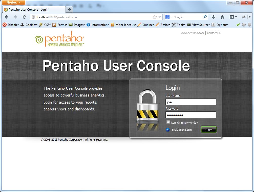
Enter the standard username / password ( joe / password ) and get inside. Now you need to install the olap-client, which will, in fact, display our requests to it. The paid version of Pentaho has its own client, for CE we used the Saiku plugin.
We go to the Pentaho Marketplace item of the top menu, install Saiku Analytics.
That's all for now, it's time to prepare data for analytics.
Preparation of fact tables and measurements
Pentaho is a ROLAP implementation of OLAP technology, i.e. all the data that we will analyze is stored in ordinary relational tables, except perhaps, in some way, prepared in advance. Therefore, all we need is to create the necessary tables.
I will say a little about the subject area for which we needed statistics. There is a website, there are customers, and there are tickets that these customers can write. Also with comments, yes. And our support breaks all these tickets on different topics, projects, countries. And so we needed, for example, to find out how many tickets on the subject “Delivery” came from each project from Germany over the past month. And break it all down by admin, i.e. see who is from support and how many such tickets processed, etc. etc.
All such slices and OLAP technology allows. I won’t talk about OLAP in detail. We assume that the reader is familiar with the concepts of OLAP cube, measurements and measures, and in general terms imagines what it is and what it is eaten with.
Of course, I will not analyze the real data of real clients as an example, and for this purpose I will use my small site with football statistics. There is little practical benefit from this, but as a sample - it is.
So there is a players table . Let's try to find all kinds of useful and not very statistics: the number of players in each country, the number of players in the lineup, the number of active players, the number of Russian midfielders aged 30 to 40 years. Well, something like that ...
So where did I stop? And, exactly, the preparation of tables. There are several ways: to recreate all the tables with your hands and bare SQL nicks, or use the Pentaho Data Integration utility (PDI, also known as Kettle) - a Pentaho complex component responsible for the process of extracting, converting and uploading data (ETL). It allows you to establish a connection with a specific database and, using a lot of different tools, prepare the tables we need. Download it . We drop the mysql connector into the lib folder and run PDI through Spoon.bat .
First, let's collect the heart of our statistics - the table of players. Initially, its structure looks something like this:
CREATE TABLE IF NOT EXISTS `player` (
  `id` int(11) unsigned NOT NULL AUTO_INCREMENT COMMENT 'ID',
  `name` varchar(40) DEFAULT NULL COMMENT 'Имя',
  `patronymic` varchar(40) DEFAULT NULL COMMENT 'Отчество',
  `surname` varchar(40) DEFAULT NULL COMMENT 'Фамилия',
  `full_name` varchar(255) DEFAULT NULL COMMENT 'Полное имя',
  `birth_date` date NOT NULL COMMENT 'Дата рождения',
  `death_date` date DEFAULT NULL COMMENT 'Дата смерти',
  `main_country_id` int(11) unsigned NOT NULL COMMENT 'ID страны',
  `birthplace` varchar(255) DEFAULT NULL COMMENT 'Место рождения',
  `height` tinyint(3) unsigned DEFAULT NULL COMMENT 'Рост',
  `weight` tinyint(3) unsigned DEFAULT NULL COMMENT 'Вес',
  `status` enum('active','inactive') NOT NULL DEFAULT 'active' COMMENT 'Статус игрока - играет, завершил карьеру и т.д.',
  `has_career` enum('no','yes') NOT NULL DEFAULT 'no' COMMENT 'Есть ли подробная статистика по карьере',
  PRIMARY KEY (`id`),
  KEY `name` (`name`),
  KEY `surname` (`surname`),
  KEY `birth_date` (`birth_date`),
  KEY `death_date` (`death_date`),
  KEY `has_stat` (`has_career`),
  KEY `main_country_id` (`main_country_id`),
  KEY `status` (`status`),
  KEY `full_name_country_id` (`full_name_country_id`)
) ENGINE=InnoDB  DEFAULT CHARSET=utf8 COMMENT='Игроки' AUTO_INCREMENT=1;
Some of the fields (name, surname, patronymic, full_name or birthplace, for example) are not needed for statistics. Fields of the Enum type (status, has_career) need to be placed in separate dimension tables, and simply enter the identifiers of foreign keys in the main table.

So, let's get started: File> New> Job (Ctrl + Alt + N). The workspace of the job opens. Go to the View tab, create a new database connection ( Database connections> New ): drive the server, database, user and password, give the connection some name (I have fbplayers) and save ( c: \ Pentaho \ biserver-ce \ pentaho -solutions \ jobs \ fbplayers.kjb ).
Create a transformation ( File> New> Transformation , Ctrl + N). Save it as prepare_tables.ktr. In the same way as with the job, we add a connection to the database for transformation. Done.
Go to the View tab and expand the Input section. Select the Data Grid tool . It is well suited if you need to move some fields with a small number of possible options into separate related tables. So, pull the Data Grid to the workspace and open it for editing with a double click. We drive in the name of this transformation step ( Player Status ), we begin to set the structure of this table (Meta tab) and the data itself (Data tab). We have 2 fields in the structure:
1. Name - id, Type - Integer, Decimal - 11
2. Name - status, Type - String, Length - 10.
In the Data tab, we drive 2 lines: 1 - active, 2 - inactive.
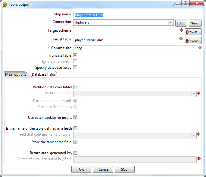
Go to the Output section and pull out the Table Output element. Double click, set the item name as Player Status Dim . The connection should appear in the next line. In the Target Table field, write the name of the table that will be created in the database to store the status of the players: player_status_dim. We put the checkbox Truncate Table. We connect the input and output elements: click on the Player Status and, while holding the Shift button, drag the mouse to Player Status Dim. The link should appear as an arrow connecting these elements.
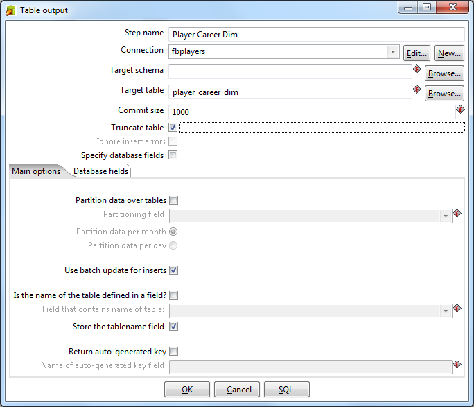
The same thing needs to be turned with a flag for a career ( Player Career ):
1. Name - id, Type - Integer, Decimal - 11
2. Name - has_career, Type - String, Length - 3.
In the Data tab, drive 2 lines: 1 - no, 2 - yes.
Similarly, we collect the output player Career Dim table .
Now we will place the player’s birth date in a separate measurement table. By and large, Pentaho allows you to use the date directly in the fact table, initially we did this with the data in our subject area. But there were several problems:
1. if you need to split 2 different fact tables (for example, Players and Coaches) by date of birth, then you need a common dimension (Dimension) for them;
2. when dividing the date in the fact table itself into component parts of a function such as extract or year (month, ...) it will be applied to each row of the table to obtain the year, month, etc. What is not ice.
So, for these reasons, we redid our original structure and created a table with all the unique values of time, leaving the clock as a minimum level. For our test example, there will be no such detailing, only years, months and days will be.
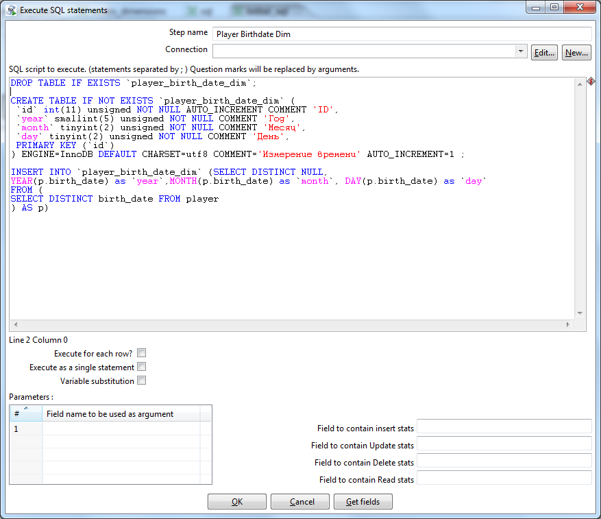
Create a new transformation ( initial_sql ). Do not forget about the connection. From the collection of items, select Scripting> Execute SQL Script . We write the date picker into it:
DROP TABLE IF EXISTS `player_birth_date_dim`;
CREATE TABLE IF NOT EXISTS `player_birth_date_dim` (
  `id` int(11) unsigned NOT NULL AUTO_INCREMENT COMMENT 'ID',
  `year` smallint(5) unsigned NOT NULL COMMENT 'Год',
  `month` tinyint(2) unsigned NOT NULL COMMENT 'Месяц',
  `day` tinyint(2) unsigned NOT NULL COMMENT 'День',
  PRIMARY KEY (`id`)
) ENGINE=InnoDB DEFAULT CHARSET=utf8 COMMENT='Измерение времени' AUTO_INCREMENT=1 ;
INSERT INTO `player_birth_date_dim`
(SELECT DISTINCT NULL, YEAR(p.birth_date) as `year`,
MONTH(p.birth_date) as `month`, DAY(p.birth_date) as `day`
FROM (
  SELECT DISTINCT birth_date FROM player
) AS p)
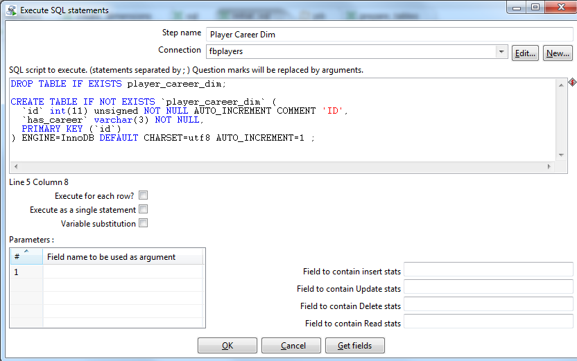
Right here, in this transformation, we create 2 more SQL scripts - to create the table Player Career Dim and Player Status Dim:
DROP TABLE IF EXISTS player_career_dim;
CREATE TABLE IF NOT EXISTS `player_career_dim` (
  `id` int(11) unsigned NOT NULL AUTO_INCREMENT COMMENT 'ID',
  `has_сareer` varchar(3) NOT NULL,
  PRIMARY KEY (`id`)
) ENGINE=InnoDB DEFAULT CHARSET=utf8 AUTO_INCREMENT=1 ;
DROP TABLE IF EXISTS player_status_dim;
CREATE TABLE IF NOT EXISTS `player_status_dim` (
  `id` int(11) unsigned NOT NULL AUTO_INCREMENT COMMENT 'ID',
  `status` varchar(10) NOT NULL,
  PRIMARY KEY (`id`)
) ENGINE=InnoDB DEFAULT CHARSET=utf8 AUTO_INCREMENT=1 ;

We proceed to the main part of our mission - the assembly of the fact table. Create a transformation ( player_fact.ktr ). They didn’t forget about the connection, right? From the Input tab, we throw Table Input, from Output - Table Output, respectively. In the Table Input we write a cool SQL nickname:
SELECT
p.id AS player_id,
dd.id AS birth_date_id,
p.main_country_id,
p.height,
p.weight,
CASE p.status
    WHEN 'active' THEN 1
    WHEN 'inactive' THEN 2
END as status_id,
CASE p.has_career
    WHEN 'no' THEN 1
    WHEN 'yes' THEN 2
END as has_career_id
FROM player AS `p`
INNER JOIN player_birth_date_dim AS dd
ON YEAR(p.birth_date) = dd.`year`
AND MONTH(p.birth_date) = dd.`month` AND DAY(p.birth_date) = dd.`day`
In Table Output, specify the table name - player_fact . We connect the source and resulting tables with an arrow.
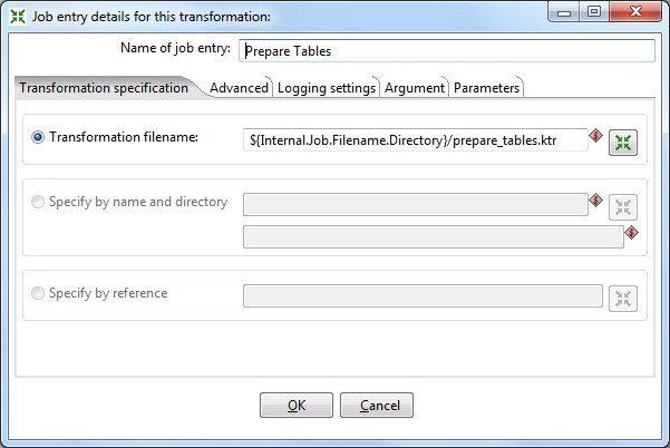
Again we go to our job. From the General tab, add a new transformation. Open it, give the name Prepare Tables and specify the path to our saved transformation prepare_tables.ktr .
We do the same with the Initial SQL and Player Fact transformations .
We drop the Start button on the form and connect the elements in the following sequence: Start> Initial SQL> Prepare Tables> Load Player Fact .
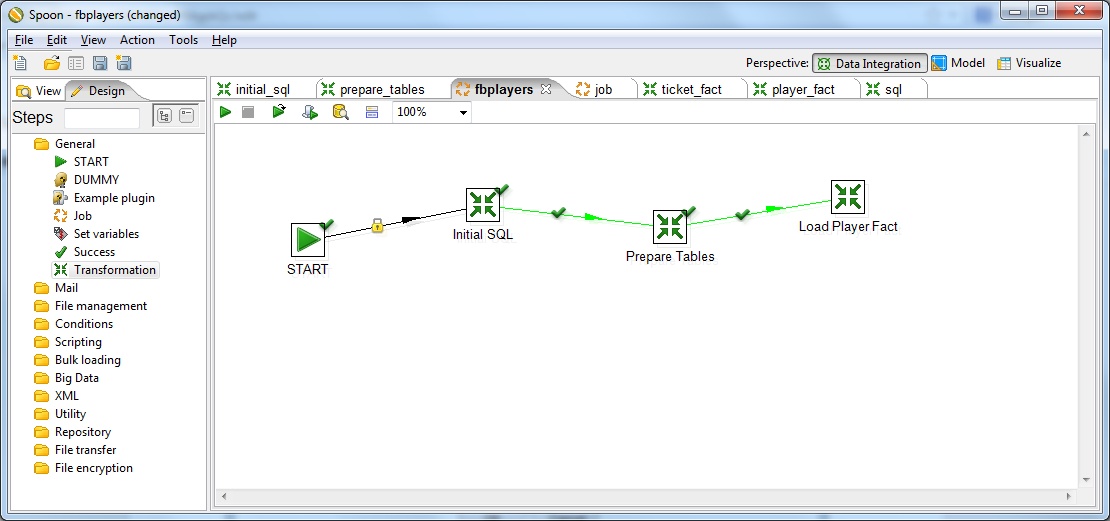
Now you can try to run the task. In the toolbar, click the green triangle. If our hands were straight enough, then next to each of our elements we will see a green tick. You can go to your server and verify that the plates are actually created. If something went wrong, then the log will show all our sins.
Create a cube and publish it to the server
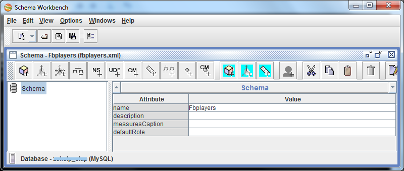
Now that we have the prepared data, we will finally take up OLAP. Pentaho has a Schema Workbench utility to create olap cubes . Download, unpack, drop the mysql connector into the drivers folder, run workbench.bat .
Immediately go to the menu Options> Connection . We enter our database connection parameters.
Getting started: File> New> Schema . Immediately save the scheme (I have fbplayers.xml ). Set the name of the scheme.
Using the context menu of the circuit, create a cube. We will call it the name of the entity whose statistics we will consider, i.e. Player Get .
Inside the cube, we indicate the table, which will be our fact table: player_fact.
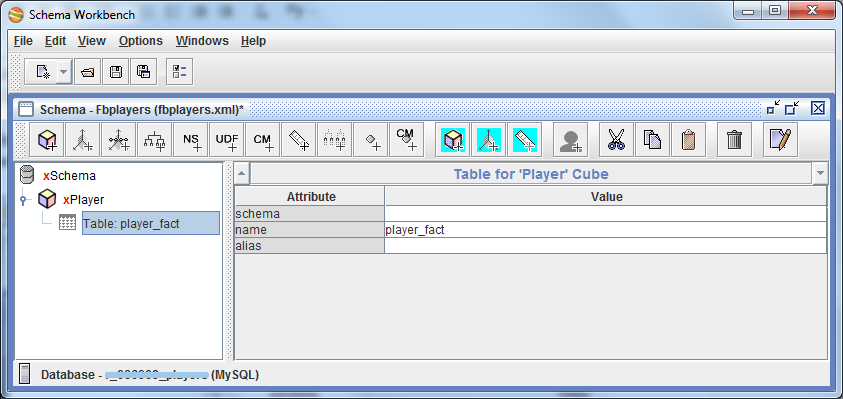
If you select the Player cube, the red line at the bottom of the right pane will tell us that Dimensions should be set in the cube, i.e. those parameters by which data slices will be performed.
There are 2 ways to set a dimension for a cube: directly inside it (via Add Dimension ) and inside the circuit (Add Dimension for the circuit plus Add Dimension Usage for the cube itself). We used the second option in our statistics, because it allows one dimension to be applied to several fact tables at once (to several cubes). We then combined these cubes into a virtual cube, which allowed us to display statistics for several cubes simultaneously.
In our test project, we will also use the second method, unless we create virtual cubes.
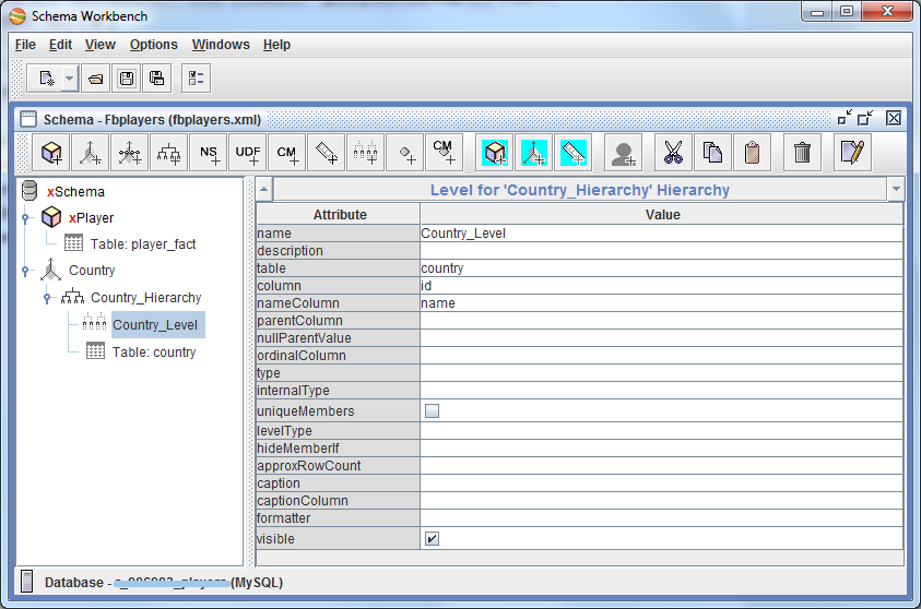
So, add the first dimension (by country). Create a schema dimension, give it the name Country . There is already 1 hierarchy inside it, we will give it the name Country_Hierarchy . In this hierarchy, we add a table that stores the values of the Country dimension, i.e. country.
This is my regular mysql table with a list of countries with the following structure:
CREATE TABLE IF NOT EXISTS `country` (
  `id` int(11) unsigned NOT NULL AUTO_INCREMENT COMMENT 'ID',
  `name` varchar(40) NOT NULL COMMENT 'Название',
  `english_name` varchar(40) NOT NULL COMMENT 'Название на английском',
  `iso_alpha_3` varchar(3) NOT NULL COMMENT 'Трехбуквенный код ISO 3166-1',
  PRIMARY KEY (`id`),
  KEY `name` (`name`),
  KEY `england_name` (`english_name`)
) ENGINE=InnoDB  DEFAULT CHARSET=utf8 COMMENT='Страны' AUTO_INCREMENT=1 ;
After that we add to the hierarchy 1 level (Add Level). We call it Country_Level and associate the fact table with this dimension table: set the table field to country, column to id, nameColumn to name. Those. this means that when comparing the country ID from the fact table, the country ID from the country table will return the name of the country as a result (for readability). The remaining fields, in principle, can be left blank.
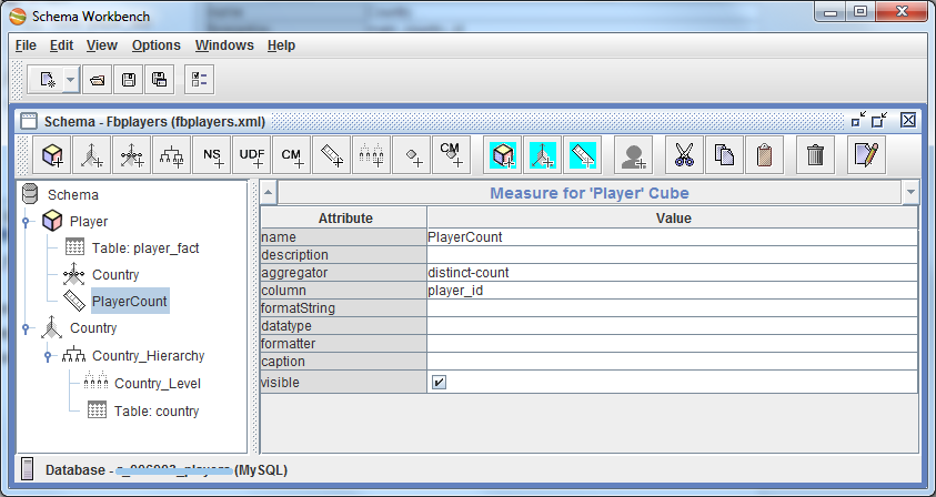
Now we can return to the Player cube and assign it the newly created dimension (via Add Dimension Usage). We set the name (Country), source is our created measurement Country (in the drop-down list it will be the only one so far), and the foreignKey field is main_country_id, i.e. this tells Pentaho that when he sees some main_country_id in the fact table, he accesses the dimension table (Country) on the specified column (id) and substitutes the name_name for main_country_id. Something like this ... It

remains only to indicate to the cube that we actually want to aggregate something)) Add a measure ( Add Measure ) to the cube . Let's give it the name PlayerCount, the aggregator - distinct-count and the field by which we will aggregate - player_id. Done!
Let's dwell on this for a short while and check what we have conjured here. We launch the Pentaho web-muzzle:
localhost:8080/pentaho(do not forget about start-pentaho.bat). Go to File> Manage> Data Sources . Click the add new source button. Select the type - Database Table (s). The most important thing we need here is to create a new Connection. We set the name (Fbplayers) and drive our data to access the database. After saving Connection, click Cancel everywhere, we don’t need anything else. Next, we need to publish the created scheme on the Pentaho server: File> Publish . Set url:
localhost:8080/pentahoand enter the password for the publication. This password is set in the file c: \ Pentaho \ biserver-ce \ pentaho-solutions \ system \ publisher_config.xml. Set this password to 123, for example, the user and password are standard - joe / password. If everything is fine, then after that a window for selecting a folder should be displayed, where to save our scheme. Enter the name of the connection that we created in the last step (Fbplayers) in the "Pentaho or JNDI Source" field. Create a schema folder and save the file to it. If everything went fine, we should see a joyful window:
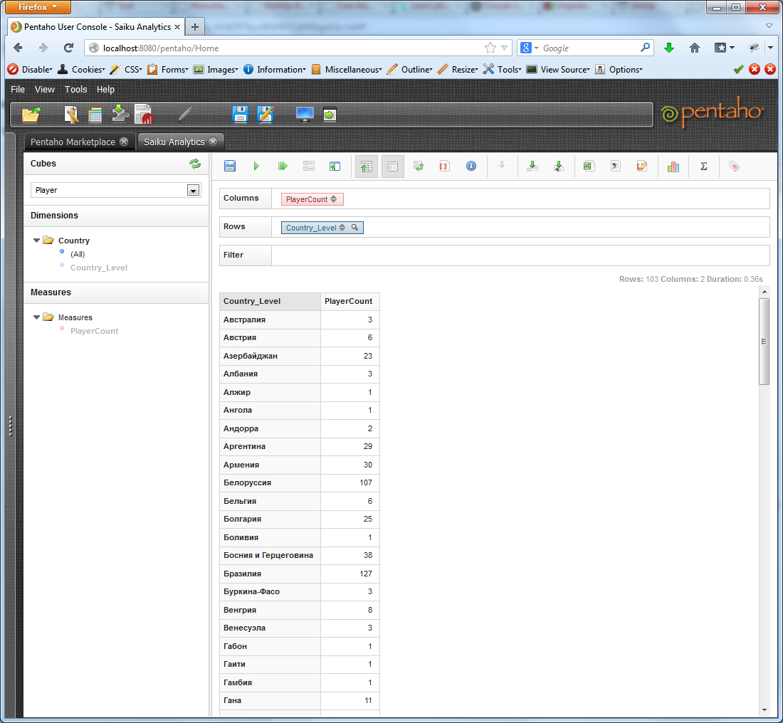
Let's go look! We go to the web-face, open Saiku, select our cube from the drop-down list. We see the Country dimension and the PlayerCount measure appear. Drag Country_Level in the Rows field, PlayerCount in Columns. By default, the button for automatic query execution is pressed on the Saiku panel. Usually it is necessary to squeeze it before dragging measurements and measures, but this is not important. If automatic execution is disabled, click the Run button. Rejoice!
But if suddenly instead of beautiful data you saw a message like “EOFException: Can not read response from server. Expected to read 4 bytes, read 0 bytes before connection was unexpectedly lost ”, don’t worry - it happens, just click Run one more time or two.
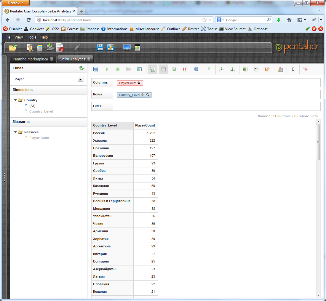
By clicking on the arrows on the measure button, we can sort the resulting selection in descending or ascending order.
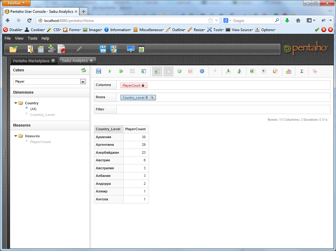
While we have a little data, let's see what is still available. You can limit the output, say, only by country to the letter A:
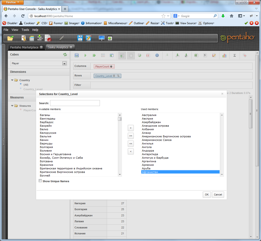
We get:
You can see the graphs. This is usually beautiful if there is little data in the sample.
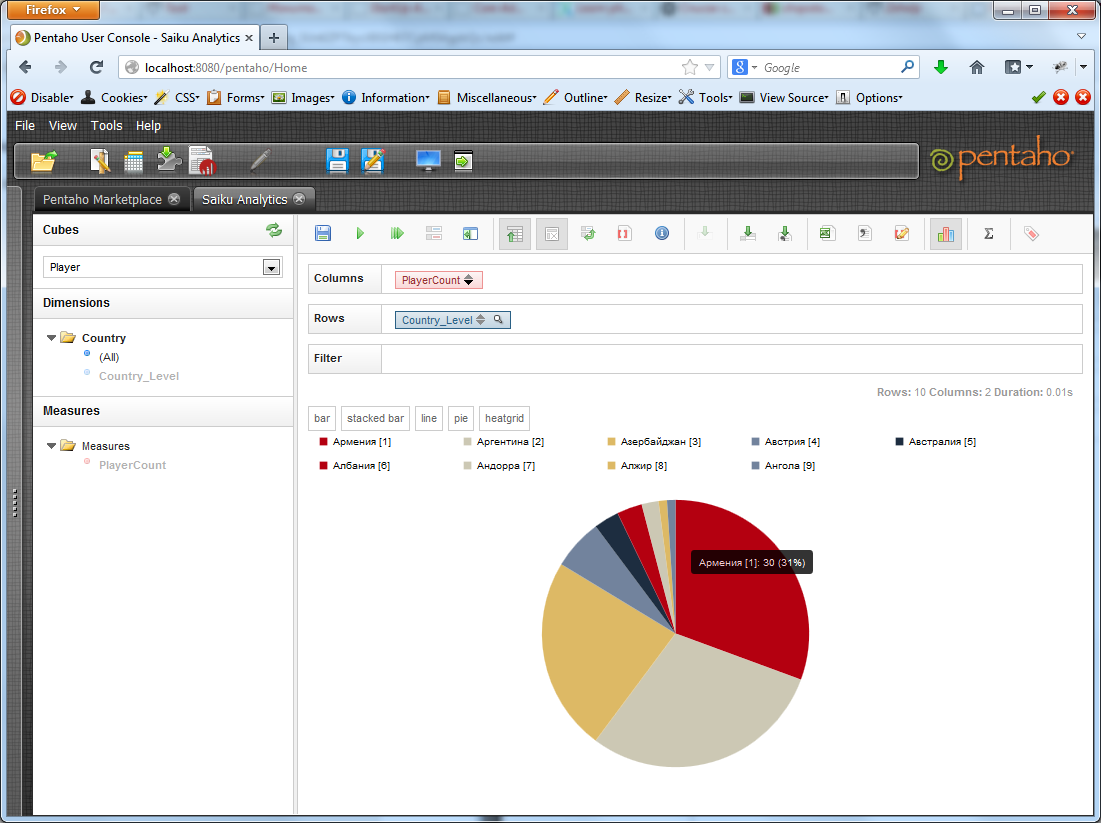
You can see the statistics for the sample: minimum, maximum indicator, average value, etc. You can upload all this property to xls or csv. Also, the request thrown by us using the constructor can be saved on the server, so that later we can return to it.
So, the essence is clear. Let's create a couple more dimensions. In principle, measurements by player status and career are no different from measurements by country. And the result in both cases will be only 2 lines (active / inactive and has / no).
The situation with the hierarchy of the Date type is much more interesting. We will create it now. We return to the Workbench, add a new dimension ( BirthDate ). Instead of StandardDimension, we set the parameter TimeDimension . There is already a hierarchy here. Add a dimension table - player_birth_date_dim .
Add the first level - Year. Set table = player_birth_date_dim, column = id, levelType = TimeYears. For this level, add the Key Expression property with the value of `year`.
Add the second level - Month . Set table = player_birth_date_dim, column = id, levelType = TimeMonths. For this level, add the Key Expression property with the value of `month`, Caption Expression with the value of“ CONCAT (`year`, ',', MONTHNAME (STR_TO_DATE (` month`, '% m'))) ”.
Add the third level - Day . Set table = player_birth_date_dim, column = id, levelType = TimeDays. For this level, add the Caption Expression property with the value “CONCAT (LPAD (` day`, 2, 0), '.', LPAD (`month`, 2, 0), '.',` Year`) ".
Add the created dimension to the cube, specifying bith_date_id as a foreignKey.
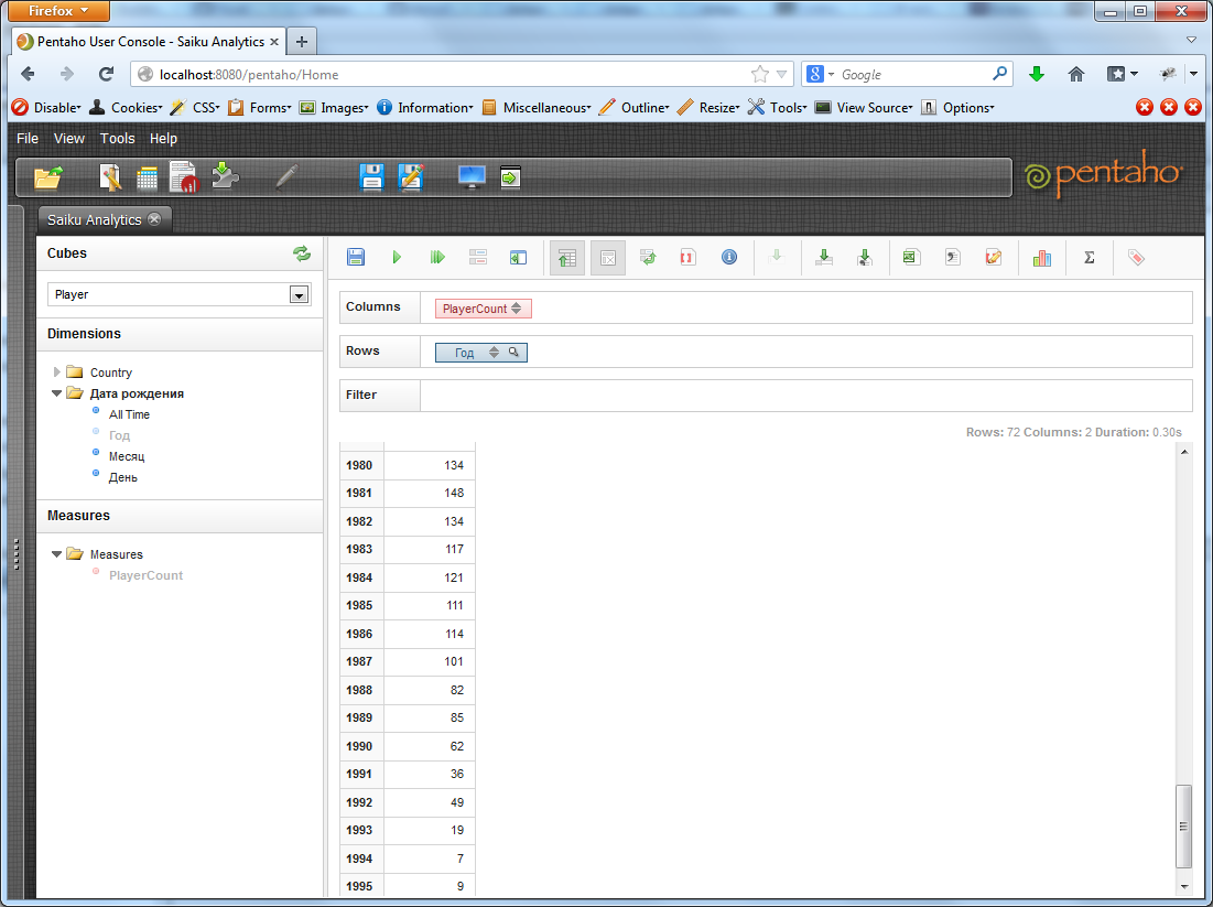
Publish. Let's try to break all the players by year of birth.
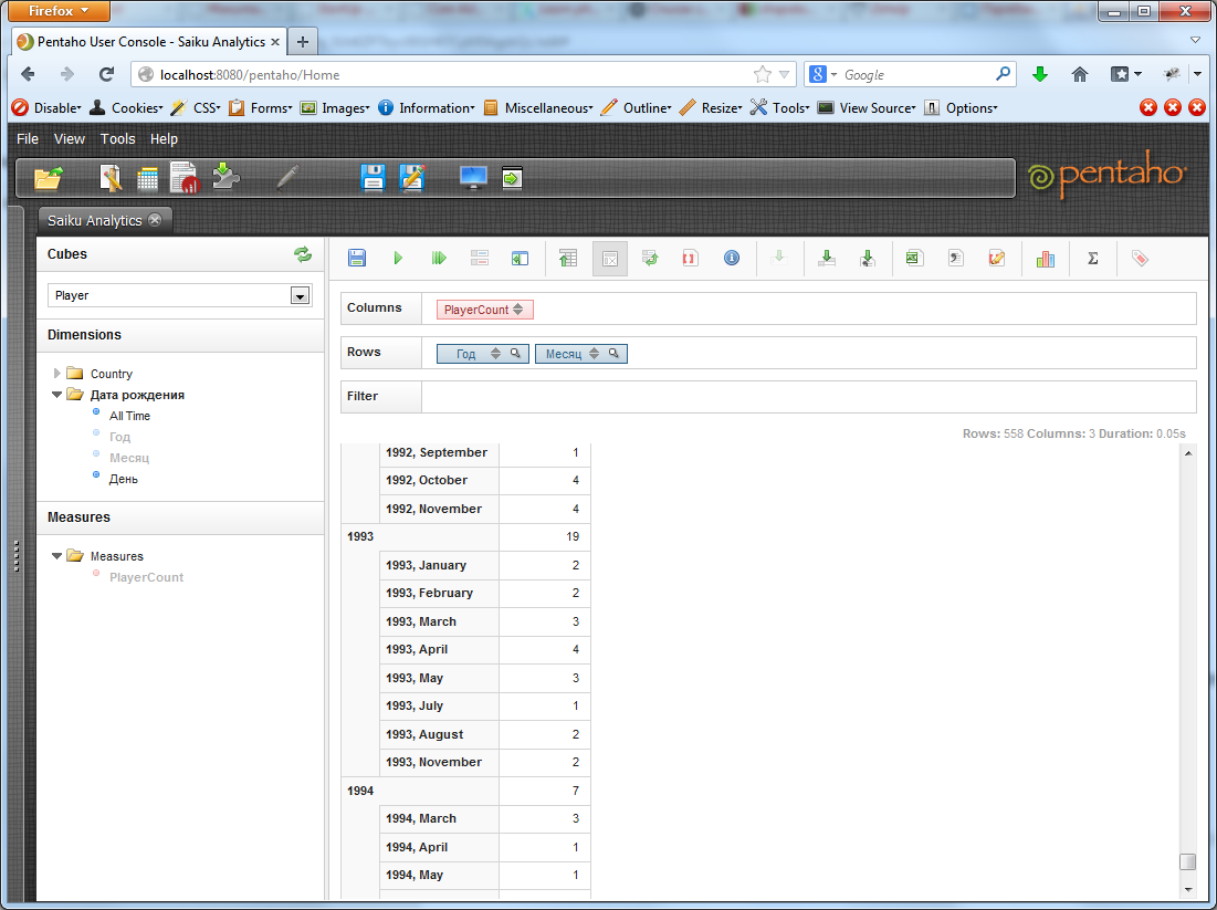
And now we’ll add the “Month” parameter to the “Year” parameter. Pentaho will break each of the years into months and calculate the number of players born in a particular month of each year. By default, only monthly data is displayed, but if you press the “Hide Parents” button in the toolbar, you can see the total number of players for a given year.
But the main strength of Pentaho, and indeed the entire OLAP, in fact, is not in such simple samples, but in slices from several measurements at the same time. Those. for example, we find the number of players in each country born after 1990.
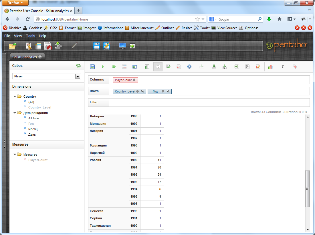
As the number of metrics increases, queries can become more complex and pointy, reflecting a specific static need.
This concludes our long-long article. I hope this tutorial will help someone take a fresh look at OLAP solutions or maybe even introduce these solutions in their organizations.