Sea battle as a recognition task
Hello, Habr!
Continuing the week of naval combat, I want to offer another way to build the optimal shooting strategy. It uses a tree representation of strategy, which is very common in game theory. The presentation of the problem in the form of a solution table is borrowed from the theory of tests, which was popular in the 70s of the last century and was used, in particular, for monitoring and diagnosing faults in electronic circuits. This method allows you to find the optimal strategy, but it has a very large computational complexity. Alas, the game on the 10x10 field could not be analyzed.
To begin with, we will get a convenient way to present the strategy in the form of a decision tree. For example, here's how you can shoot a cruiser and two boats on a 3x3 field.
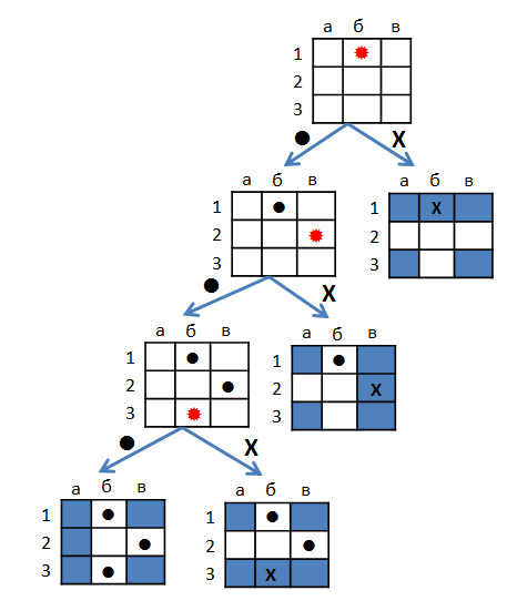
At the tops of the tree is a playing field with shots already taken. The current shot is marked in red. The result of the shot is attributed to the ribs: miss (.) Or hit (x). The leaves show the location of the ships. The strategy can be described in words like this. First, shoot at b1 . If we hit, it becomes clear how the ships are located, and it remains to finish them off. If not, shoot at B2 . If we fall, everything is clear again. If we miss, there are two options for the location, and a shot in b3 brings final clarity.
It is clear that any shooting strategy can be described in this way, paper would have been enough. But in order to find a good strategy, you need to formalize what we really want. Note that the strategy describes the player’s actions “for all occasions,” but a specific game with its location of the ships is described by a path in the tree from the root to one of the leaves. Having finished to the end and won, we will get as many times as there were pipes on the ships of the enemy. You can reformulate the rules like this: each of the players shoots until the enemy squadron is completely destroyed, and then the one who has fewer misses wins. So a good strategy is different from a bad amount of misses. And now we have two possibilities.
You can evaluate the strategy by how many misses will be made in the worst case. Then, of the two strategies, the one with the maximum number of misses from the root to the leaf is minimal. And we can assume that the enemy chooses a location by chance with equal probability, and try to reduce the expected number of misses. Then, of the two strategies, one that has the smallest total in all paths from the root of each leaf leaf will be the best. For example, our strategy allows guaranteed destruction of ships by making no more than three misses, and the expected number of misses is (3 + 2 + 1 + 0) / 4 = 1.5.
By the way, you can try to find a strategy that will be the best in both senses. Sounds tempting? Alas, both problems are too similar to the NP-hard problem of covering the setthat promises us the lack of easy decision algorithms. But, stocking up with patience and machine time, we still try to do something.
Let's imagine the task in the form of a so-called decision table. We will build a rectangular table in which the columns correspond to the cells of the playing field, and the rows correspond to all kinds of options for the location of the ships. The cell of the table at the intersection of the row and column contains the sign "X" if there is a ship in the given location of the ships in this cell of the playing field, and "." otherwise. For example, here is a table that describes four possible options for the location of the cruiser and two boats in the 3x3 field (each line on the right is assigned a cell in which the middle of the cruiser is located - in our example, it uniquely determines the location of the ships).
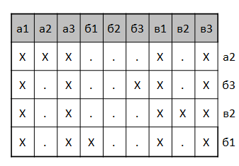
Looking at the table, you can understand that it makes no sense to shoot B2 , because in no configuration there is a ship. Shots at a1 ,a3 , b1 , b3 guarantees hit, but does not provide additional information about the location of the ships. They can be performed at the beginning to intimidate the enemy. A shot at each of the remaining cells when hit uniquely determines the line, and when missed, reduces the number of hypotheses by one. You can imagine this process as deleting from the table rows that contradict the accumulated information.
An approximate greedy algorithm builds a tree starting at the root. The algorithm selects a column of the table (cell for the shot), so that the proportion of rows that have a ship in this cell is as close as possible to 1/2. The selected cell is attributed to the root of the tree, two edges corresponding to a miss / hit are drawn from the root, two new vertices are suspended at the ends of the edges. Each of the new vertices gets a subtable, in which the lines that contradict the results of the first shot are crossed out. The same procedure is applied to each leaf until all the resulting tables contain only one row. The corresponding vertices become leaves, and the algorithm terminates.
Another algorithm uses dynamic programming. He analyzes a huge graph of sub-tables, but ensures that the solution found is optimal. Unfortunately, a detailed story about him deserves a separate post. Somehow I will gather my strength and write, and now I propose to believe in its existence and move on to the experimental part.
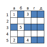
The number of configurations (1.85 * 10 15 ), voiced by the respected Mrrl , caught me in the process of writing the code and pretty much cooled my ardor. Thinking, I decided to bring the matter to the end, while reducing the size of the field. The exact algorithm agreed to work out the task of firing at a squadron of one cruiser, two destroyers and three boats on a 5x5 field. The number of possible configurations is only 1428, but the graph of subtasks consists of an impressive 10 191 257 peaks and 214 464 800 edges. The optimal algorithm allows you to destroy the squadron, making no more than seven misses, and on average allows 4.51 misses. The figure below shows how you can determine the position of ships by five misses (i.e., when implementing the rightmost branch of the decision tree).
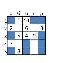
The greedy algorithm for the same task built a strategy that allowed 11 misses in the worst case, with an expected number of misses of 5.46. The figure below shows the miss shooting strategy (the rightmost branch of the decision tree).
The classic greedy algorithm worked badly. I think he would do a good job of minimizing the length of the path in the tree, and the number of misses clearly requires a different empiric choice of cells for the shot. The exact algorithm overcame the problem with half the ships on the quarter of the field, so there is nothing to boast about. A little warms the soul that for this small task, we now know the same number of misses for the optimal strategy (7 in the worst case, 4.51 on average). I would be glad if this helps colleagues building approximate algorithms.
1) The considered problem differs from the classic “sea battle” in that instead of “killed” the player gives the answer “hit”. The introduction of the third answer does not allow us to describe the subtask only with a list of locations that are compatible with previous shots and apply dynamic programming for the solution. I can’t imagine how to search for the optimal algorithm for the classical problem, unless by direct enumeration with the exception of proven non-optimal branches.
2) A greedy algorithm that selects at each step a column with a maximum number of characters X(i.e., choosing the cage for the shot with the highest probability of finding the ship), shows a result close to optimal: 8 misses in the worst case and 4.595 on average. The introduction of the answer “killed” significantly improves the performance: 4 misses in the worst case and 2.04 misses on average.
Thanks Mrrl for the additions.
Continuing the week of naval combat, I want to offer another way to build the optimal shooting strategy. It uses a tree representation of strategy, which is very common in game theory. The presentation of the problem in the form of a solution table is borrowed from the theory of tests, which was popular in the 70s of the last century and was used, in particular, for monitoring and diagnosing faults in electronic circuits. This method allows you to find the optimal strategy, but it has a very large computational complexity. Alas, the game on the 10x10 field could not be analyzed.
Decision tree
And when Great Britain, and then Germany, built the dreadnoughts, a war between them became inevitable. Because, in addition to questions about the tactics of using new ships, which at least somehow could be answered speculatively, there was one, which theoretically was absolutely impossible to answer. It sounded like this: “WHOSE DARNISHES ARE BETTER ?!”(A free quote from the play “Dreadnought” by E. Grishkovets)
To begin with, we will get a convenient way to present the strategy in the form of a decision tree. For example, here's how you can shoot a cruiser and two boats on a 3x3 field.

At the tops of the tree is a playing field with shots already taken. The current shot is marked in red. The result of the shot is attributed to the ribs: miss (.) Or hit (x). The leaves show the location of the ships. The strategy can be described in words like this. First, shoot at b1 . If we hit, it becomes clear how the ships are located, and it remains to finish them off. If not, shoot at B2 . If we fall, everything is clear again. If we miss, there are two options for the location, and a shot in b3 brings final clarity.
It is clear that any shooting strategy can be described in this way, paper would have been enough. But in order to find a good strategy, you need to formalize what we really want. Note that the strategy describes the player’s actions “for all occasions,” but a specific game with its location of the ships is described by a path in the tree from the root to one of the leaves. Having finished to the end and won, we will get as many times as there were pipes on the ships of the enemy. You can reformulate the rules like this: each of the players shoots until the enemy squadron is completely destroyed, and then the one who has fewer misses wins. So a good strategy is different from a bad amount of misses. And now we have two possibilities.
You can evaluate the strategy by how many misses will be made in the worst case. Then, of the two strategies, the one with the maximum number of misses from the root to the leaf is minimal. And we can assume that the enemy chooses a location by chance with equal probability, and try to reduce the expected number of misses. Then, of the two strategies, one that has the smallest total in all paths from the root of each leaf leaf will be the best. For example, our strategy allows guaranteed destruction of ships by making no more than three misses, and the expected number of misses is (3 + 2 + 1 + 0) / 4 = 1.5.
By the way, you can try to find a strategy that will be the best in both senses. Sounds tempting? Alas, both problems are too similar to the NP-hard problem of covering the setthat promises us the lack of easy decision algorithms. But, stocking up with patience and machine time, we still try to do something.
Decision table and strategy building algorithms
Let's imagine the task in the form of a so-called decision table. We will build a rectangular table in which the columns correspond to the cells of the playing field, and the rows correspond to all kinds of options for the location of the ships. The cell of the table at the intersection of the row and column contains the sign "X" if there is a ship in the given location of the ships in this cell of the playing field, and "." otherwise. For example, here is a table that describes four possible options for the location of the cruiser and two boats in the 3x3 field (each line on the right is assigned a cell in which the middle of the cruiser is located - in our example, it uniquely determines the location of the ships).

Looking at the table, you can understand that it makes no sense to shoot B2 , because in no configuration there is a ship. Shots at a1 ,a3 , b1 , b3 guarantees hit, but does not provide additional information about the location of the ships. They can be performed at the beginning to intimidate the enemy. A shot at each of the remaining cells when hit uniquely determines the line, and when missed, reduces the number of hypotheses by one. You can imagine this process as deleting from the table rows that contradict the accumulated information.
An approximate greedy algorithm builds a tree starting at the root. The algorithm selects a column of the table (cell for the shot), so that the proportion of rows that have a ship in this cell is as close as possible to 1/2. The selected cell is attributed to the root of the tree, two edges corresponding to a miss / hit are drawn from the root, two new vertices are suspended at the ends of the edges. Each of the new vertices gets a subtable, in which the lines that contradict the results of the first shot are crossed out. The same procedure is applied to each leaf until all the resulting tables contain only one row. The corresponding vertices become leaves, and the algorithm terminates.
Another algorithm uses dynamic programming. He analyzes a huge graph of sub-tables, but ensures that the solution found is optimal. Unfortunately, a detailed story about him deserves a separate post. Somehow I will gather my strength and write, and now I propose to believe in its existence and move on to the experimental part.
Experiment
The theorist decides what he can, how he needs to, and the practitioner decides what he needs, how he can.
The number of configurations (1.85 * 10 15 ), voiced by the respected Mrrl , caught me in the process of writing the code and pretty much cooled my ardor. Thinking, I decided to bring the matter to the end, while reducing the size of the field. The exact algorithm agreed to work out the task of firing at a squadron of one cruiser, two destroyers and three boats on a 5x5 field. The number of possible configurations is only 1428, but the graph of subtasks consists of an impressive 10 191 257 peaks and 214 464 800 edges. The optimal algorithm allows you to destroy the squadron, making no more than seven misses, and on average allows 4.51 misses. The figure below shows how you can determine the position of ships by five misses (i.e., when implementing the rightmost branch of the decision tree).

The greedy algorithm for the same task built a strategy that allowed 11 misses in the worst case, with an expected number of misses of 5.46. The figure below shows the miss shooting strategy (the rightmost branch of the decision tree).

Summary
The classic greedy algorithm worked badly. I think he would do a good job of minimizing the length of the path in the tree, and the number of misses clearly requires a different empiric choice of cells for the shot. The exact algorithm overcame the problem with half the ships on the quarter of the field, so there is nothing to boast about. A little warms the soul that for this small task, we now know the same number of misses for the optimal strategy (7 in the worst case, 4.51 on average). I would be glad if this helps colleagues building approximate algorithms.
Update
1) The considered problem differs from the classic “sea battle” in that instead of “killed” the player gives the answer “hit”. The introduction of the third answer does not allow us to describe the subtask only with a list of locations that are compatible with previous shots and apply dynamic programming for the solution. I can’t imagine how to search for the optimal algorithm for the classical problem, unless by direct enumeration with the exception of proven non-optimal branches.
2) A greedy algorithm that selects at each step a column with a maximum number of characters X(i.e., choosing the cage for the shot with the highest probability of finding the ship), shows a result close to optimal: 8 misses in the worst case and 4.595 on average. The introduction of the answer “killed” significantly improves the performance: 4 misses in the worst case and 2.04 misses on average.
Thanks Mrrl for the additions.
