Solving the problem of finding the camera’s installation angles over the road using different methods in Wolfram Mathematica. Part 2
Last time, we downloaded data from a file, sorted it into a structure, got the equations of the vehicle’s motion tracks and graphically displayed these data: Part 1
In this article, using one of the methods, we will find statistically a point in the vicinity of which the vehicle’s motion tracks intersect.
Description of one of the ways to find the point of interest to us
In this method, we find all the intersection points of the graphs - vehicle movement tracks, find the mathematical expectation of this data and the variance.
Finding all track intersection points
We define the number of equations in the list with the equations:
length = Length[numeq];Create an empty list in which we will write the coordinates of the intersection points of the tracks:
rootlist = {};Now you need to write a loop. which will solve the linear equations we have in pairs and find the coordinates of their intersection and write to the prepared list ::
Do[Do[rootlist = Append[rootlist, List[ x /. Solve[numeq[[j]] == numeq[[i]], x][[1]], numeq[[j]] /. Solve[numeq[[j]] == numeq[[i]], x][[1]] ] ] , {i, 1 + j, length}], {j, 1, length}]At each pass of the cycle, we add to the
rootlistlist consisting of the coordinate xand yintersection jand the iequation, while the x coordinate is found as:, x /. Solve[numeq[[j]] == numeq[[i]], x][[1]]and
Solve[numeq[[j]] == numeq[[i]], x]returns a list The roots of this equation:,
{{x -> 2586.14}}and our record selects the first root, it is the only one here, and performs the substitution, i.e. instead of x, the operator is
/.substituted with its value x -> 2586.14.expr /. x > value- in the expr expression, instead of the variable x, its value value is substituted .
Thus, the coordinate X of the intersection of two tracks is found, a similar action is also performed to find the coordinate Y, only the root value is now substituted into one of the equations, in this case, in index j, and this can also be an equation with index i:
numeq[[j]] /. Solve[numeq[[j]] == numeq[[i]], x][[1]]Next, round off the value of our points to the whole:
rootlist = Round[rootlist];Now we have a list of track intersection points and can start statistical processing.
The list looks like this:
{{2586, -910}, {2716, -1014}, {2718, -1015}, {3566, -1697}, {2697, -999}, {2957, -1207}, ... }Statistical processing of results
Define the mat expectation of the X coordinate of the intersection list:
Xmed = Mean[rootlist[[All, 1]]] // N2532.7Mean[data]- returns the average value of the data data. N[expr, n]- returns the result of the calculation of the expression expr with an accuracy of n digits after the decimal point x // f- Postfix form for f[x]Define the variance of the coordinate X of the intersection list:
sX = StandardDeviation[rootlist[[All, 1]]] // N81038.5StandardDeviation[data]- returns the standard deviation of the data, speaking Russian - the function returns sigma, well, or standard deviation. Let us determine the same characteristics for the Y coordinate of the intersection:
Ymed = Mean[rootlist[[All, 2]]] // NsY = StandardDeviation[rootlist[[All, 2]]] // N-699.907106488From the obtained mathematical expectation data, it is already possible to determine the desired values - the angle of rotation of the camera relative to the edge of the curb:,
Xangle = Xang Xmed/Xlen - Xang/2 // N8.02449and the angle of the camera relative to the trajectories of vehicles
Yangle = Abs[Yang Ymed/Ylen - Yang/2] // N9.38796In general, such a large value of the standard deviation is somewhat confusing. we’ll build a histogram to see the distribution of quantities and find out why this happens:
Histogram[{rootlist[[Range[length], 1]], rootlist[[Range[length], 2]]},100, AspectRatio -> 1]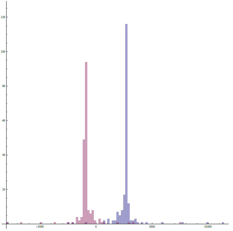
Histogram[list,bspec]- builds a histogram of the list listwith the number of columns bspecFrom this histogram, it can be seen that there are intersection points that are far from the mathematical expectation of the value.
Let’s try not to take into account points that do not satisfy the following condition:
X coordinate of the point must lie within the [horizontal resolution of the camera; 2 horizontal resolutions of the camera] The
Y coordinate of the point must lie within [- 2 vertical resolutions of the camera; 0.5 camera vertical resolution]
To do this, we write the following:
length = Length[rootlist];rlist = {};Do[If[ -Xlen < rootlist[[i, 1]] < 2 Xlen && -2 Ylen < rootlist[[i, 2]] < 0.5 Ylen, rlist = Append[rlist, rootlist[[i]]]] , {i, length}]If[condition, t, f]- returnstif the result of the calculation conditionis True, and will give f, if the result is FalseAnd[p,q,...]or p && q && ...- logical addition - the operation "And"; Let us evaluate the expectation mat and standard deviation of the resulting filtered sample:
Xmed = Mean[rlist[[Range[length], 1]]] // NYmed = Mean[rlist[[Range[length], 2]]] // NsX = StandardDeviation[rlist[[Range[length], 1]]] // NsY = StandardDeviation[rlist[[Range[length], 2]]] // N2628.84-928.819353.112457.717The resulting scatter of the filtered sample is less than that of the full sample. The desired angles can be determined in the same way as in the case of the full sample.
Graphical representation of the results.
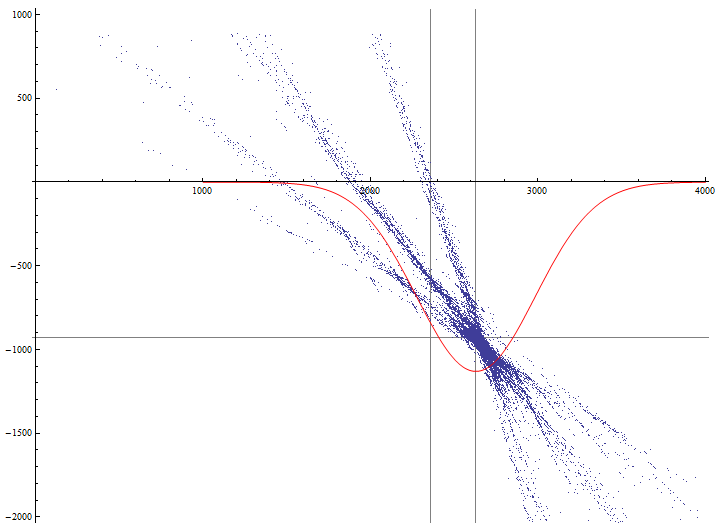
Now we will display on one graph the intersection points along the filtered sample and the distribution function of the X coordinate of the intersection points:
lp = ListPlot[rlist, PlotStyle -> PointSize[0.0005], GridLines -> {{Xlen, Xmed}, {Ylen, Ymed}}, AspectRatio -> Automatic];dp = Plot[-1000000 PDF[NormalDistribution[Xmed, sX], x], {x,1000, 4000}, PlotStyle -> {Red}];Show[lp, dp, PlotRange -> {{0, 4000}, {-2000, 1000}}, AxesOrigin -> {0, 0}]PDF[dist,x]- returns the value of the probability density of the distribution with the argument xand the given distribution law distNormalDistribution[mu,sigma]- the normal distribution I cheated a little and set the coefficient -1000000 to make the graph clear.
What's next?
In the next article, I will show another way to determine the intersection point, based on filtering equations and finding subsets within the set.
Only registered users can participate in the survey. Please come in.
Should I write articles on linear data processing in Mathematica?
- 84.2% Yes 32
- 15.7% No 6
- 0% Custom option in comments 0