Robust estimators
- From the sandbox
- Tutorial
I want to apologize right away, I learned about robust estimators from English literature, so some terms are direct tracing paper from English, it may well be that in Russian-language literature the topic of robust evaluations has some kind of its own stable momentum.
While studying at the university, the course of statistics that we were taught (and this was more than 15 years ago) was the most typical one: an introduction through probability theory and frequently occurring distributions. Since then nothing more has been left in my head about this semester course. It seems to me that much is given much better in the course of statistical physics. Much later, life confronted me with medical physics, where statistical methods are one of the main tools for analyzing data obtained, for example, using NMR tomography. This is the first time I have come across the term robust statistics and robust estimators. Immediately make a reservation, I will show only simple examples of the use of robust estimators and give links to literature, those interested can easily deepen and expand their knowledge using the list of literature at the end of this article. Let's take a look at the simplest example most frequently encountered to demonstrate a reliable estimate in a sample. Suppose student Vasya sits at a physical workshop and writes down the testimony of a certain device:
4.5
4.1
5.2
5.5
3.9
4.3
5.7
6.0
45
47
The device doesn’t work very accurately, plus Vasya is distracted by talking with a Lena, a roommate. As a result, Vasily does not put a decimal point in the last two entries, and voila, we have a problem.
Step one, we arrange our sample in ascending order and calculate the mean value of
mean = 13.12. It is
immediately clear that the average value is far from the real average due to the last two outliers that fell into the sample. The easiest way to estimate the average without taking into account the effect of emissions is the median
median = 5.35
Thus, the simplest robust estimator is the median; indeed, we can see that up to 50% of the data can be “polluted” with various kinds of outliers, but the estimate of the median will not change. Using this simple example, several concepts can be introduced at once: what is the robustness in statistics (stability of estimates with respect to outliers in the data), how much the used estimator is robust (how much it is possible to “pollute” the data without significantly changing the estimates obtained) [1]. Can the median score be improved? Of course, you can enter an even more reliable estimator known as the absolute deviation from the median (median absolute deviation or MAD)
MAD = median (| xi-median [xj] |)
in the case of a normal distribution, a numerical factor is introduced before the MAD, which allows one to keep the estimate unchanged. As you can see, the stability of MAD is also 50%.
Robust estimators found huge practical application in linear regressions. In the case of a linear dependence (x, y), it is often necessary to obtain well-conditioned estimates of such a dependence (often in the case of multivariate regression)
y = Bx + E ,
where B can already be a matrix of coefficients, E is some noise spoiling our measurements, and x is a set parameters (vector), which we actually want to evaluate using the measured values of y(vector). The simplest and most well-known way to do this is the least squares method (LSM) [2]. In principle, it is very easy to make sure that the MNC is not a robust estimator and its robust reliability is 0%, because even a single outlier can significantly change the estimate. One of the most mathematical beautiful tricks to improve the score is called least trimmed squares or the method of “trimmed” squares (MUK). His idea is to trivially modify the original OLS, in which the number of estimates used is cut, i.e.: the
original LSN
MUK
where r_i are already ordered errors of estimates (y - O (x)) , i.e. r_1. Again, one can easily verify that the minimum trimming factor, which allows a reliable estimate of h = N / 2 + p ( p is the number of independent variables plus one), i.e. robust evaluation reliability can again be almost 50%. Actually, everything is quite simple with the MUK, except for one non-trivial question related to the choice of h. The first sighting method of choice can be characterized as “by sight”. If the sample where we conduct the regression is not very large, then the number of outliers can be estimated and the trimming factor selected by trying several close values, especially if the estimate does not change with decreasing / increasing. However, there are more stringent selection criteria [3,4], which, unfortunately, lead to a noticeable increase in the calculation time even in the case of linear regressions.
We briefly list other well-known estimators that are often used in the literature [1]:
1) least median squares (method of median squares)
2) M-, R-, S-, Q- estimators, estimators based on a certain evaluation function (for example, OLS can also be called an M-estimator), and
various variations in error estimation (moments cutting off hyperplanes, etc.).
3) Estimators for nonlinear regressions [5]
Paragraph two in this list is somewhat inaccurate, because for convenience, many estimators that are quite different in nature are collected in one heap.
As a simple but very interesting application of robust estimates, we give a robust estimate of the diffusion tensor in NMR tomography [6]. One of the interesting applications in NMR tomography is diffusion measurements on water molecules, which are subject to Brownian motion in the brain. However, due to various restrictions (movement along neuro-fibers, in dendrides, inside and outside cells, etc.) they have different diffusion parameters. Making measurements in six different directions (the diffusion tensor is positive definite, i.e. we need to know only 6 of its elements), we can restore the tensor itself, through the well-known signal decay model. Spatial directions are encoded by gradient coils in a pulsed sequence. We can imagine the diffusion tensor as an ellipsoid,
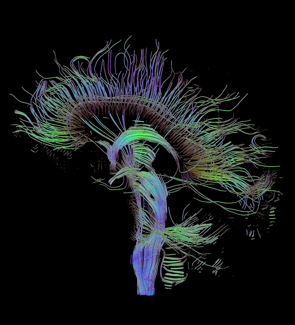
) The threads are ordered tensors that are approximated by a certain curve (through the well-known Runge-Kutta method). This approach is called streamline [7].
However, measurements of this kind are richest in various kinds of artifacts (compared to other types of images) due to heartbeat, respiratory movement of the chest, head movement during measurements, different tics, table trembling due to often switching magnetic gradients, etc. . Thus, the reconstructed diffusion tensor can have noticeable deviations from the present values and, as a result, the wrong direction in the case of its pronounced anisotropy. This does not allow the use of the obtained nerve fiber tracks as a reliable source of information about the device of nerve connections or to plan surgical operations. In fact, the diffusion tensor approach is not used to restore the image of nerve fibers, so most patients need not worry so far.
The mathematical theory of robust estimators is quite interesting, because in many cases it is based on already known approaches (this means that most of the rigorous and dry theories are already known), but has additional properties that can significantly complement and improve the estimated results. If we return to the already mentioned OLS, then the introduction of weighting factors allows us to obtain robust estimates in the case of linear regression. The next step is to change the weighting factors by introducing iterations in the estimates, as a result we get the well-known iteratively reweighted least squares approach [2].
I hope readers unfamiliar with robust statistics have got some idea about robust estimators, and acquaintances saw interesting applications for their knowledge.
Literature
1. Rousseeuw PJ, Leroy AM, Robust regression and outlier detection. Wiley, 2003.
2. Bjoerck A, Numerical methods for least squares problems. SIAM, 1996.
3. Agullo, J. New algorithm for computing the least trimmed squares regression estimator. Computational statistics & data analysis 36 (2001) 425-439.
4. Hofmann M, Gatu C, Kontoghiorghes EJ. An exact least trimmed squares algorithm for a range of coverage values. Journal of computational and graphical statistics 19 (2010) 191-204.
5. Motulsky HJ, Brown RE. Detecting outliers when fitting data with nonlinear regression - a new method based on robust nonlinear regression and the false discovery rate. BMC Bioinfromatics 7 (2006) 123.
6. Change LC, Jones DK, Pierpaoli C. RESTORE: Robust estimation of tensors by oulier rejection. Magnetic Resonance in Medicine 53 (2005) 1088-1085.
7. Jones DK, Diffusion MRI: Theory, Methods and Applications. Oxford University Press, 2010.
While studying at the university, the course of statistics that we were taught (and this was more than 15 years ago) was the most typical one: an introduction through probability theory and frequently occurring distributions. Since then nothing more has been left in my head about this semester course. It seems to me that much is given much better in the course of statistical physics. Much later, life confronted me with medical physics, where statistical methods are one of the main tools for analyzing data obtained, for example, using NMR tomography. This is the first time I have come across the term robust statistics and robust estimators. Immediately make a reservation, I will show only simple examples of the use of robust estimators and give links to literature, those interested can easily deepen and expand their knowledge using the list of literature at the end of this article. Let's take a look at the simplest example most frequently encountered to demonstrate a reliable estimate in a sample. Suppose student Vasya sits at a physical workshop and writes down the testimony of a certain device:
4.5
4.1
5.2
5.5
3.9
4.3
5.7
6.0
45
47
The device doesn’t work very accurately, plus Vasya is distracted by talking with a Lena, a roommate. As a result, Vasily does not put a decimal point in the last two entries, and voila, we have a problem.
Step one, we arrange our sample in ascending order and calculate the mean value of
mean = 13.12. It is
immediately clear that the average value is far from the real average due to the last two outliers that fell into the sample. The easiest way to estimate the average without taking into account the effect of emissions is the median
median = 5.35
Thus, the simplest robust estimator is the median; indeed, we can see that up to 50% of the data can be “polluted” with various kinds of outliers, but the estimate of the median will not change. Using this simple example, several concepts can be introduced at once: what is the robustness in statistics (stability of estimates with respect to outliers in the data), how much the used estimator is robust (how much it is possible to “pollute” the data without significantly changing the estimates obtained) [1]. Can the median score be improved? Of course, you can enter an even more reliable estimator known as the absolute deviation from the median (median absolute deviation or MAD)
MAD = median (| xi-median [xj] |)
in the case of a normal distribution, a numerical factor is introduced before the MAD, which allows one to keep the estimate unchanged. As you can see, the stability of MAD is also 50%.
Robust estimators found huge practical application in linear regressions. In the case of a linear dependence (x, y), it is often necessary to obtain well-conditioned estimates of such a dependence (often in the case of multivariate regression)
y = Bx + E ,
where B can already be a matrix of coefficients, E is some noise spoiling our measurements, and x is a set parameters (vector), which we actually want to evaluate using the measured values of y(vector). The simplest and most well-known way to do this is the least squares method (LSM) [2]. In principle, it is very easy to make sure that the MNC is not a robust estimator and its robust reliability is 0%, because even a single outlier can significantly change the estimate. One of the most mathematical beautiful tricks to improve the score is called least trimmed squares or the method of “trimmed” squares (MUK). His idea is to trivially modify the original OLS, in which the number of estimates used is cut, i.e.: the
original LSN
min \sum_{i=1}^N r_i^2, MUK
min \sum_{i=1}^h {r_i^2}_{1:N}, where r_i are already ordered errors of estimates (y - O (x)) , i.e. r_1
We briefly list other well-known estimators that are often used in the literature [1]:
1) least median squares (method of median squares)
min median r_i^2 2) M-, R-, S-, Q- estimators, estimators based on a certain evaluation function (for example, OLS can also be called an M-estimator), and
various variations in error estimation (moments cutting off hyperplanes, etc.).
3) Estimators for nonlinear regressions [5]
Paragraph two in this list is somewhat inaccurate, because for convenience, many estimators that are quite different in nature are collected in one heap.
As a simple but very interesting application of robust estimates, we give a robust estimate of the diffusion tensor in NMR tomography [6]. One of the interesting applications in NMR tomography is diffusion measurements on water molecules, which are subject to Brownian motion in the brain. However, due to various restrictions (movement along neuro-fibers, in dendrides, inside and outside cells, etc.) they have different diffusion parameters. Making measurements in six different directions (the diffusion tensor is positive definite, i.e. we need to know only 6 of its elements), we can restore the tensor itself, through the well-known signal decay model. Spatial directions are encoded by gradient coils in a pulsed sequence. We can imagine the diffusion tensor as an ellipsoid,
) The threads are ordered tensors that are approximated by a certain curve (through the well-known Runge-Kutta method). This approach is called streamline [7].
However, measurements of this kind are richest in various kinds of artifacts (compared to other types of images) due to heartbeat, respiratory movement of the chest, head movement during measurements, different tics, table trembling due to often switching magnetic gradients, etc. . Thus, the reconstructed diffusion tensor can have noticeable deviations from the present values and, as a result, the wrong direction in the case of its pronounced anisotropy. This does not allow the use of the obtained nerve fiber tracks as a reliable source of information about the device of nerve connections or to plan surgical operations. In fact, the diffusion tensor approach is not used to restore the image of nerve fibers, so most patients need not worry so far.
The mathematical theory of robust estimators is quite interesting, because in many cases it is based on already known approaches (this means that most of the rigorous and dry theories are already known), but has additional properties that can significantly complement and improve the estimated results. If we return to the already mentioned OLS, then the introduction of weighting factors allows us to obtain robust estimates in the case of linear regression. The next step is to change the weighting factors by introducing iterations in the estimates, as a result we get the well-known iteratively reweighted least squares approach [2].
I hope readers unfamiliar with robust statistics have got some idea about robust estimators, and acquaintances saw interesting applications for their knowledge.
Literature
1. Rousseeuw PJ, Leroy AM, Robust regression and outlier detection. Wiley, 2003.
2. Bjoerck A, Numerical methods for least squares problems. SIAM, 1996.
3. Agullo, J. New algorithm for computing the least trimmed squares regression estimator. Computational statistics & data analysis 36 (2001) 425-439.
4. Hofmann M, Gatu C, Kontoghiorghes EJ. An exact least trimmed squares algorithm for a range of coverage values. Journal of computational and graphical statistics 19 (2010) 191-204.
5. Motulsky HJ, Brown RE. Detecting outliers when fitting data with nonlinear regression - a new method based on robust nonlinear regression and the false discovery rate. BMC Bioinfromatics 7 (2006) 123.
6. Change LC, Jones DK, Pierpaoli C. RESTORE: Robust estimation of tensors by oulier rejection. Magnetic Resonance in Medicine 53 (2005) 1088-1085.
7. Jones DK, Diffusion MRI: Theory, Methods and Applications. Oxford University Press, 2010.