KNN classifier
kNN stands for k Nearest Neighbor or k Nearest Neighbors - this is one of the simplest classification algorithms, also sometimes used in regression tasks. Due to its simplicity, it is a good example from which you can begin your acquaintance with the field of Machine Learning. This article describes an example of writing the code for such a classifier in python, as well as visualizing the results.
Classification taskin machine learning, this is the task of assigning an object to one of the predefined classes based on its formalized features. Each of the objects in this problem is represented as a vector in N-dimensional space, each dimension in which is a description of one of the features of the object. Suppose we need to classify monitors: measurements in our parameter space will be the diagonal in inches, aspect ratio, maximum resolution, HDMI interface, cost, etc. The case of classifying texts is somewhat more complicated, they usually use a term-document matrix ( description on machinelearning .ru ).
To train the classifier, you must have a set of objects for which classes are predefined. This set is calledtraining sample , its marking is done manually, with the involvement of specialists in the study area. For example, in the task of Detecting Insults in Social Commentary for pre-assembled tests of comments, a person puts down the opinion whether this comment is an insult to one of the participants in the discussion, the task itself is an example of binary classification. In the classification problem, there can be more than two classes (multiclass), each of the objects can belong to more than one class (intersecting).
To classify each of the objects of the test sample, the following operations must be performed sequentially:
The examples below are implemented in python. For their correct execution, in addition to python, you must have numpy , pylab and matplotlib installed . The library initialization code is as follows:
Consider the work of the classifier by example. To begin with, we need to generate data on which experiments will be made:
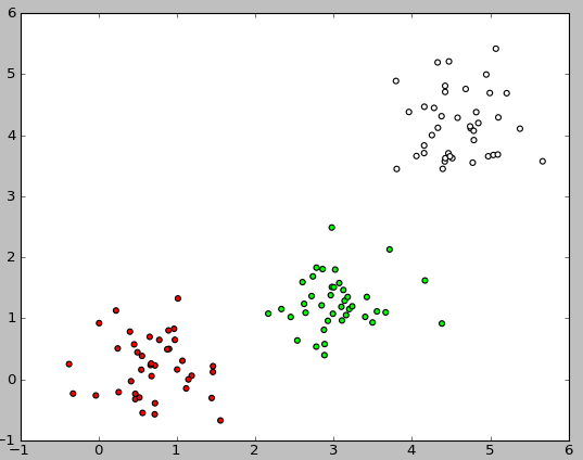
For simplicity, I chose a two-dimensional space in which the location of the mathematical expectation of a two-dimensional Gaussian with a standard deviation of 0.5 is randomly selected from 0 to 5 along each axis. The value 0.5 is chosen so that the objects turn out to be fairly well separable (the rule of three sigma ).
To look at the resulting selection, you need to run the following code:
Here is an example of the image resulting from the execution of this code:
So, we have a set of objects, for each of which a class is defined. Now we need to break this set into two parts: training selection and test selection. To do this, use the following code:
Now, having a training sample, we can implement the classification algorithm itself:
To determine the distance between objects, you can use not only the Euclidean distance: the Manhattan distance, cosine measure, Pearson's correlation criterion, etc. are also used.
Now you can evaluate how well our classifier works. To do this, we will generate the data, we will divide it into a training and test sample, we will classify the objects of the test sample and compare the real value of the class with the result of the classification:
To evaluate the quality of the classifier, various algorithms and various measures are used; more details can be found here: wiki
Now the most interesting thing remains: to show the classifier’s work graphically. In the pictures below, I used 3 classes, each with 40 elements, the value of k for the algorithm was taken to be three.
The following code was used to display these images:
kNN is one of the simplest classification algorithms, so it often turns out to be ineffective in real problems. In addition to the accuracy of the classification, the problem of this classifier is the speed of classification: if there are N objects in the training set, M objects in the test set, and the space dimension K, then the number of operations for classifying the test set can be estimated as O (K * M * N). Nevertheless, the kNN algorithm is a good example to get started with Machine Learning.
1. The method of nearest neighbors on Machinelearning.ru
2. The vector model on Machinelearning.ru
3. Book on Information Retrieval
4. Description of the method of nearest neighbors in the framework of scikit-learn
5. Book “Programming collective intelligence”
Classification taskin machine learning, this is the task of assigning an object to one of the predefined classes based on its formalized features. Each of the objects in this problem is represented as a vector in N-dimensional space, each dimension in which is a description of one of the features of the object. Suppose we need to classify monitors: measurements in our parameter space will be the diagonal in inches, aspect ratio, maximum resolution, HDMI interface, cost, etc. The case of classifying texts is somewhat more complicated, they usually use a term-document matrix ( description on machinelearning .ru ).
To train the classifier, you must have a set of objects for which classes are predefined. This set is calledtraining sample , its marking is done manually, with the involvement of specialists in the study area. For example, in the task of Detecting Insults in Social Commentary for pre-assembled tests of comments, a person puts down the opinion whether this comment is an insult to one of the participants in the discussion, the task itself is an example of binary classification. In the classification problem, there can be more than two classes (multiclass), each of the objects can belong to more than one class (intersecting).
Algorithm
To classify each of the objects of the test sample, the following operations must be performed sequentially:
- Calculate the distance to each of the objects in the training set
- Select k objects of the training set, the distance to which is minimum
- The class of a classified object is the class most often found among k nearest neighbors
The examples below are implemented in python. For their correct execution, in addition to python, you must have numpy , pylab and matplotlib installed . The library initialization code is as follows:
import random
import math
import pylab as pl
import numpy as np
from matplotlib.colors import ListedColormap
Initial data
Consider the work of the classifier by example. To begin with, we need to generate data on which experiments will be made:
#Train data generator
def generateData (numberOfClassEl, numberOfClasses):
    data = []
    for classNum in range(numberOfClasses):
        #Choose random center of 2-dimensional gaussian
        centerX, centerY = random.random()*5.0, random.random()*5.0
        #Choose numberOfClassEl random nodes with RMS=0.5
        for rowNum in range(numberOfClassEl):
            data.append([ [random.gauss(centerX,0.5), random.gauss(centerY,0.5)], classNum])
    return data
For simplicity, I chose a two-dimensional space in which the location of the mathematical expectation of a two-dimensional Gaussian with a standard deviation of 0.5 is randomly selected from 0 to 5 along each axis. The value 0.5 is chosen so that the objects turn out to be fairly well separable (the rule of three sigma ).
To look at the resulting selection, you need to run the following code:
def showData (nClasses, nItemsInClass):
    trainData      = generateData (nItemsInClass, nClasses)
    classColormap  = ListedColormap(['#FF0000', '#00FF00', '#FFFFFF'])
    pl.scatter([trainData[i][0][0] for i in range(len(trainData))],
               [trainData[i][0][1] for i in range(len(trainData))],
               c=[trainData[i][1] for i in range(len(trainData))],
               cmap=classColormap)
    pl.show()
showData (3, 40)
Here is an example of the image resulting from the execution of this code:
Getting training and test samples
So, we have a set of objects, for each of which a class is defined. Now we need to break this set into two parts: training selection and test selection. To do this, use the following code:
#Separate N data elements in two parts:
#	test data with N*testPercent elements
#	train_data with N*(1.0 - testPercent) elements
def splitTrainTest (data, testPercent):
    trainData = []
    testData  = []
    for row in data:
        if random.random() < testPercent:
            testData.append(row)
        else:
            trainData.append(row)
    return trainData, testData
Classifier Implementation
Now, having a training sample, we can implement the classification algorithm itself:
#Main classification procedure
def classifyKNN (trainData, testData, k, numberOfClasses):
    #Euclidean distance between 2-dimensional point
    def dist (a, b):
        return math.sqrt((a[0] - b[0])**2 + (a[1] - b[1])**2)
    testLabels = []
    for testPoint in testData:
        #Claculate distances between test point and all of the train points
        testDist = [ [dist(testPoint, trainData[i][0]), trainData[i][1]] for i in range(len(trainData))]
        #How many points of each class among nearest K
        stat = [0 for i in range(numberOfClasses)]
        for d in sorted(testDist)[0:k]:
            stat[d[1]] += 1
        #Assign a class with the most number of occurences among K nearest neighbours
        testLabels.append( sorted(zip(stat, range(numberOfClasses)), reverse=True)[0][1] )
    return testLabels
To determine the distance between objects, you can use not only the Euclidean distance: the Manhattan distance, cosine measure, Pearson's correlation criterion, etc. are also used.
Execution examples
Now you can evaluate how well our classifier works. To do this, we will generate the data, we will divide it into a training and test sample, we will classify the objects of the test sample and compare the real value of the class with the result of the classification:
#Calculate classification accuracy
def calculateAccuracy (nClasses, nItemsInClass, k, testPercent):
    data = generateData (nItemsInClass, nClasses)
    trainData, testDataWithLabels = splitTrainTest (data, testPercent)
    testData = [testDataWithLabels[i][0] for i in range(len(testDataWithLabels))]
    testDataLabels = classifyKNN (trainData, testData, k, nClasses)
    print "Accuracy: ", sum([int(testDataLabels[i]==testDataWithLabels[i][1]) for i in range(len(testDataWithLabels))]) / float(len(testDataWithLabels))
To evaluate the quality of the classifier, various algorithms and various measures are used; more details can be found here: wiki
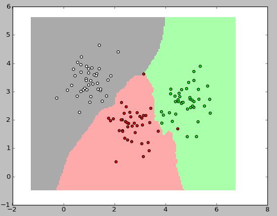
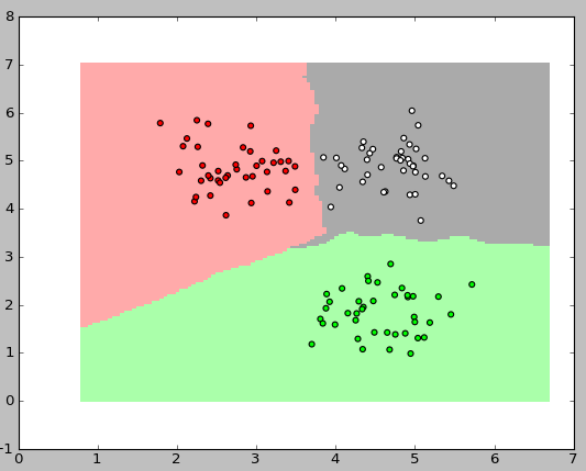
Now the most interesting thing remains: to show the classifier’s work graphically. In the pictures below, I used 3 classes, each with 40 elements, the value of k for the algorithm was taken to be three.
The following code was used to display these images:
#Visualize classification regions
def showDataOnMesh (nClasses, nItemsInClass, k):
    #Generate a mesh of nodes that covers all train cases
    def generateTestMesh (trainData):
        x_min = min( [trainData[i][0][0] for i in range(len(trainData))] ) - 1.0
        x_max = max( [trainData[i][0][0] for i in range(len(trainData))] ) + 1.0
        y_min = min( [trainData[i][0][1] for i in range(len(trainData))] ) - 1.0
        y_max = max( [trainData[i][0][1] for i in range(len(trainData))] ) + 1.0
        h = 0.05
        testX, testY = np.meshgrid(np.arange(x_min, x_max, h),
                                   np.arange(y_min, y_max, h))
        return [testX, testY]
    trainData      = generateData (nItemsInClass, nClasses)
    testMesh       = generateTestMesh (trainData)
    testMeshLabels = classifyKNN (trainData, zip(testMesh[0].ravel(), testMesh[1].ravel()), k, nClasses)
    classColormap  = ListedColormap(['#FF0000', '#00FF00', '#FFFFFF'])
    testColormap   = ListedColormap(['#FFAAAA', '#AAFFAA', '#AAAAAA'])
    pl.pcolormesh(testMesh[0],
                  testMesh[1],
                  np.asarray(testMeshLabels).reshape(testMesh[0].shape),
                  cmap=testColormap)
    pl.scatter([trainData[i][0][0] for i in range(len(trainData))],
               [trainData[i][0][1] for i in range(len(trainData))],
               c=[trainData[i][1] for i in range(len(trainData))],
               cmap=classColormap)
    pl.show()
Conclusion
kNN is one of the simplest classification algorithms, so it often turns out to be ineffective in real problems. In addition to the accuracy of the classification, the problem of this classifier is the speed of classification: if there are N objects in the training set, M objects in the test set, and the space dimension K, then the number of operations for classifying the test set can be estimated as O (K * M * N). Nevertheless, the kNN algorithm is a good example to get started with Machine Learning.
List of references
1. The method of nearest neighbors on Machinelearning.ru
2. The vector model on Machinelearning.ru
3. Book on Information Retrieval
4. Description of the method of nearest neighbors in the framework of scikit-learn
5. Book “Programming collective intelligence”