Evaluation of spatial orientation, or How not to be afraid of filters Mahoney and Majvika

Tutorial

What are we talking about

The appearance on Habré of the post about Majvik's filter was in its own way a symbolic event. Apparently, the universal enthusiasm for drones has revived interest in the problem of estimating the orientation of a body from inertial measurements. At the same time, traditional methods based on the Kalman filter have ceased to satisfy the public, either because of the high requirements for computing resources that are unacceptable for drones, or because of the complex and non-intuitive adjustment of parameters.

The post was accompanied by a very compact and efficient implementation of the C filter. However, judging by the comments, the physical meaning of this code, as well as the whole article, remained vague for someone. Well, let's face it honestly: the Madjwick filter is the most sophisticated of a group of filters based on very simple and elegant principles. I will consider these principles in my post. Code will not be here. My post is not a story about a specific implementation of an orientation estimation algorithm, but rather an invitation to invent my own variations on a given topic, which can be very much.

Orientation view

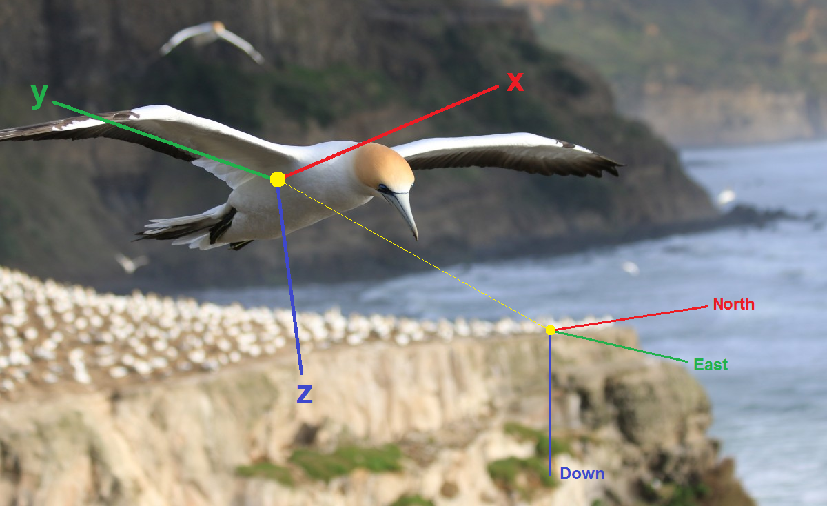
Recall the basics. To estimate the orientation of a body in space, one must first choose some parameters that, in aggregate, uniquely determine this orientation, i.e. essentially the orientation of the associated coordinate system

$inline$ relatively conditionally stationary system - for example, the NED (North, East, Down) geographic system. Then you need to make kinematic equations, i.e. express the rate of change of these parameters through the angular velocity from the gyroscopes. Finally, vector measurements from accelerometers, magnetometers, etc. need to be included in the calculation. Here are the most commonly used ways of representing orientation:

Euler angles - roll (roll,

$\ phi$ ), pitch (pitch,

$\ theta$ ) course (heading,

$\ psi$ ). This is the most obvious and most concise set of orientation parameters: the number of parameters is exactly equal to the number of rotational degrees of freedom. For these angles, one can write the Euler kinematic equations . They are very fond of theoretical mechanics, but in navigation problems they are of little use. First, knowledge of angles does not allow direct transformation of the components of a vector from a bound to a geographic coordinate system or vice versa. Secondly, with a pitch of ± 90 degrees, the kinematic equations degenerate, the list and course become uncertain.

Rotation Matrix - Matrix

$\ mathbf {C}$ 3 × 3, by which you need to multiply any vector in the associated coordinate system to get the same vector in the geographic system:

$\ mathbf {r} _ {NED} = \ mathbf {C} \ mathbf {r} _ {xyz}$ . The matrix is always orthogonal, i.e.

$\ mathbf {C} = \ mathbf {C} ^ {T}$ . The kinematic equation for it is

$\ dot {\ mathbf {C}} = \ mathbf {C} \ mathbf {\ Omega}$ .
Here

$\ mathbf {\ Omega}$ - the matrix of the components of the angular velocity measured by gyroscopes in the associated coordinate system:

$\ mathbf {\ Omega} = \ begin {bmatrix} 0 & - \ omega_ {z} & \ omega_ {y} \\ \ omega_ {z} & 0 & - \ omega_ {x} \\ - \ omega_ {y } & \ omega_ {x} & 0 \\ \ end {bmatrix}$

The rotation matrix is a little less obvious than the Euler angles, but unlike them, it allows you to directly transform vectors and does not lose meaning at any angular position. From a computational point of view, its main drawback is redundancy: for the sake of three degrees of freedom, nine parameters are entered at once, and all of them need to be updated according to the kinematic equation. The task can be slightly simplified by using the orthogonality of the matrix.

Turn quaternion is a radical, but very non-intuitive remedy against redundancy and degeneration. This is a four component object.

$\ mathbf {q} = q_ {0} + q_ {1} \ mathbf {i} + q_ {2} \ mathbf {j} + q_ {3} \ mathbf {k}$ - not a number, not a vector and not a matrix. Quaternion can be viewed from two angles. First, as the formal amount of a scalar

$q_ {0}$ and vectors

$q_ {1} \ mathbf {i} + q_ {2} \ mathbf {j} + q_ {3} \ mathbf {k}$ where

$\ mathbf {i}, \ mathbf {j}, \ mathbf {k}$ - single axis vectors (which, of course, sounds absurd). Secondly, as a generalization of complex numbers, where now not one, but three different imaginary units are used.

$\ mathbf {i}, \ mathbf {j}, \ mathbf {k}$ (which sounds no less absurd). How is quaternion related to rotation? Through the Euler theorem: a body can always be transferred from one given orientation to another with one final turn at some angle

$\ alpha$ around some axis with a guide vector

$\ mathbf {u}$ . This angle and axis can be combined into a quaternion:

$\ mathbf {q} = \ mathrm {cos} (\ alpha / 2) + \ mathbf {u} \ mathrm {sin} (\ alpha / 2)$ . Like the matrix, a quaternion can be used to directly transform any vector from one coordinate system to another:

$\ mathbf {r} _ {NED} = \ mathbf {q} \ mathbf {r} _ {xyz} {\ mathbf {q}} ^ {- 1}$ . As you can see, the quaternionic representation of the orientation also suffers from redundancy, but much less than the matrix: the extra parameter is only one. A detailed review of quaternions was already on Habré . They talked about geometry and 3D graphics. We are also interested in kinematics, since the rate of change of the quaternion must be related to the measured angular velocity. The corresponding kinematic equation is

$\ dot {\ mathbf {q}} = 1/2 \ mathbf {q} \ mathbf {\ omega}$ where is the vector

$\ mathbf {\ omega}$ also considered a quaternion with zero scalar part.

Filter schemes

The most naive approach to calculating an orientation is to arm yourself with a kinematic equation and update any set of parameters we like in accordance with it. For example, if we selected a rotation matrix, then we can write a cycle with something in the spirit C += С * Omega * dt. The result will disappoint. Gyroscopes, especially MEMS, have large and unstable zero offsets — as a result, even at complete rest, the computed orientation will have an unlimited accumulating error (drift). All the tricks invented by Mahoney, Majwick, and many others, not excluding me, were aimed at compensating for this drift by involving measurements from accelerometers, magnetometers, GNSS receivers, lags, etc. Thus was born the whole family of orientation filters, based on a simple basic principle.

The basic principle. To compensate for the orientation drift, add an additional control angular velocity to the angular velocity measured by the gyros, based on the vector measurements of other sensors. The vector of control angular velocity must strive to combine the directions of the measured vectors with their known true directions.

Here a completely different approach is concluded than in the construction of the corrective addendum of the Kalman filter. The main difference is that the controlling angular velocity is not a term, but a factor at the estimated value (matrix or quaternion). From here important advantages follow:

The rating filter can be built for the orientation itself, and not for small deviations of the orientation from that given by the gyroscopes. In this case, the estimated values will automatically satisfy all the requirements imposed by the task: the matrix will be orthogonal, the quaternion will be normalized.
The physical meaning of the control angular velocity is much clearer than the corrective term in the Kalman filter. All manipulations are done with vectors and matrices in the usual three-dimensional physical space, and not in the abstract multi-dimensional state space. This greatly simplifies the refinement and configuration of the filter, and as a bonus allows you to get rid of large-dimension matrices and heavy matrix libraries.

Now let's see how this idea is implemented in specific variants of filters.

Filter Mahoney. All the furious mathematics of the original article by Mahoney is written to justify simple equations (32). Rewrite them in our notation. If we ignore the estimation of gyro zero offsets, then two key equations will remain - the actual kinematic equation for the rotation matrix (with the controlling angular velocity in the form of

$\ mathbf {\ Omega} '$ ) and the law of formation of this very speed as a vector

$\ mathbf {\ omega} '$ . Suppose, for simplicity, that there are no accelerations or magnetic pickups, and thanks to this, we can measure acceleration due to gravity.

$- \ hat {\ mathbf {g}} _ {xyz}$ from accelerometers and magnetic field strength of the Earth

$\ hat {\ mathbf {m}} _ {xyz}$ from magnetometers. Both vectors are measured by sensors in a connected coordinate system, and in a geographic system, their position is obviously known:

$- \ mathbf {g} _ {NED}$ pointing up

$\ mathbf {m} _ {NED}$ - to magnetic north. Then the Mahoney filter equation will look like this:

$\ dot {\ mathbf {C}} = \ mathbf {C} (\ mathbf {\ Omega} + \ mathbf {\ Omega} ') \\ \ mathbf {\ omega'} = k_ {g} \ hat {\ mathbf {g}} _ {xyz} \ times \ mathbf {C} ^ {T} \ mathbf {g} _ {NED} + k_ {m} \ hat {\ mathbf {m}} _ {xyz} \ times \ mathbf {C} ^ {T} \ mathbf {m} _ {NED}$

Let's look closely at the second equation. The first item on the right is a vector product. The first factor in it is the measured acceleration of gravity, the second is the true one. Since the factors must be in the same coordinate system, the second factor is converted to the connected system by multiplying by

$\ mathbf {C} ^ {T}$ . The angular velocity, constructed as a vector product, is perpendicular to the plane of the multiplier vectors. It allows you to rotate the calculated position of the associated coordinate system until the multiplier vectors coincide in direction - then the vector product will be reset and the rotation will stop. Coefficient

$k_ {g}$ sets the stiffness of such feedback. The second term performs a similar operation with a magnetic vector. In fact, the Mahoney filter embodies a well-known thesis: knowledge of two non-collinear vectors in two different coordinate systems allows you to uniquely restore the mutual orientation of these systems. If there are more than two vectors, this will provide useful measurement redundancy. If the vector is only one, then one rotational degree of freedom (motion around this vector) cannot be fixed. For example, if only a vector is given

$- \ mathbf {g}$ then you can adjust the drift of roll and pitch, but not the course.

Of course, in the Mahoney filter it is not necessary to use the rotation matrix. There are non-canonical quaternion variants.

Virtual gyro platform. In the Mahoney filter, we attached a control angular velocity.

$\ mathbf {\ omega '}$ to related coordinate system. But you can attach it to the design position of the geographical coordinate system. The kinematic equation will then take the form

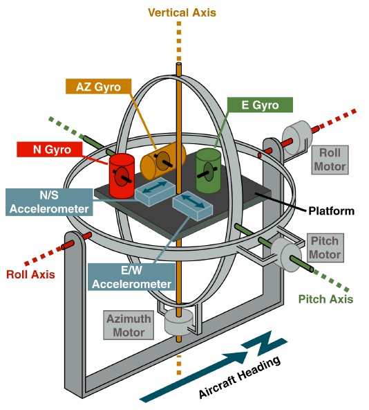
$\ dot {\ mathbf {C}} = \ mathbf {C} \ mathbf {\ Omega} - \ mathbf {\ Omega} '\ mathbf {C}$

It turns out that this approach opens the way to very fruitful physical analogies. Suffice it to recall what the gyroscopic technique began with - curshers and inertial navigation systems based on a gyrostabilized platform in a gimbal.

www.theairlinepilots.com

The task of the platform there was the materialization of the geographical coordinate system. The orientation of the carrier was measured relative to this platform by angle sensors on the suspension frames. If the gyroscopes drifted, then the platform drifted after them, and errors accumulated in the readings of the angle sensors. To eliminate these errors, feedback was introduced from accelerometers installed on the platform. For example, the deviation of the platform from the horizon around the northern axis was perceived by the accelerometer of the eastern axis. This signal allowed to set the control angular velocity

$\ mathbf {\ omega '}$ returning the platform to the horizon.

We can use the same visual concepts in our task. The written kinematic equation must then be read as follows: the rate of change in orientation is the difference between two rotational movements — the absolute movement of the carrier (the first term) and the absolute movement of the virtual gyroplatform (the second term). The analogy can be extended to the law of formation of the control angular velocity. Vector

$- \ hat {\ mathbf {g}} _ {NED} = - \ mathbf {C} \ hat {\ mathbf {g}} _ {xyz}$ personifies the testimony of accelerometers, supposedly standing on a gyro platform. Then for physical reasons you can write:

$\ omega '_ {N} = - gk_ {g} \ hat {g} _ {E}, \; \ omega '_ {E} = gk_ {g} \ hat {g} _ {N}$

It would be possible to come to the exact same result in a formal way, having made vector multiplication in the spirit of the Mahoney filter, but now not in a connected, but in a geographical coordinate system. Is it only necessary?

The first hint of a useful analogy of platform and free-form inertial navigation appears, apparently, in the ancient patent of Boeing . Then this idea was actively developed by Salychev , and more recently, by me too . The obvious advantages of this approach are:

The control angular velocity can be formed on the basis of clear physical principles.
The horizontal and course channels, which are very different in their properties and methods of correction, are naturally separated. In the filter Mahoney they are mixed.
It is convenient to compensate for the effects of accelerations by attracting GNSS data, which are issued in geographic and not related axes.
It is easy to generalize the algorithm to the case of high-precision inertial navigation, where the shape and rotation of the Earth must be taken into account. How to do it in the Mahoney scheme, I can not imagine.

Filter Majvika. Madzhvik chose a difficult path . If Mahoney, apparently, intuitively came to his decision, and then substantiated it mathematically, then Madjvik from the very beginning proved to be a formalist. He undertook to solve the optimization problem. He reasoned so. Define the orientation with a quaternion of rotation. In the ideal case, the estimated direction of some measurable vector (let it be

$- \ mathbf {g}$ ) coincides with the true. Then it will be

${\ mathbf {q}} ^ {- 1} \ mathbf {g} _ {NED} \ mathbf {q} = \ hat {\ mathbf {g}} _ {xyz}$ . In reality, this is not always achievable (especially if there are more than two vectors), but you can try to minimize the deviation

$\ mathbf {F} = {\ mathbf {q} ^ {- 1} \ mathbf {g} _ {NED} \ mathbf {q}} - \ hat {\ mathbf {g}} _ {xyz}$ from exact equality. To do this, we introduce the criterion of minimization

$E = \ frac {1} {2} | \ mathbf {F} | ^ {2} \ rightarrow \ mathrm {min}$

Minimization requires a gradient descent — moving in small steps in the direction opposite to the gradient.

$\ nabla E$ i.e. opposite to the fastest increasing function

$inline$ . By the way, Madzhvik makes a mistake: in all his works he does not enter at all

$inline$ and write insistently

$\ nabla \ mathbf {F}$ instead

$\ nabla E$ , although it actually calculates

$\ nabla E$ .

Gradient descent ultimately leads to the following condition: to compensate for orientation drift, you need to add to the rate of change of the quaternion from the kinematic equation a new negative term, proportional to

$\ nabla E$ :

$\ dot {\ mathbf {q}} = \ frac {1} {2} \ mathbf {q} \ mathbf {\ omega} - \ beta \ frac {\ nabla E} {| \ nabla E |}$

Here, Majvik deviates a bit from our “basic principle”: he adds a correction term not to the angular velocity, but to the rate of change of the quaternion, and this is not exactly the same thing. As a result, it may be that the updated quaternion will cease to be single and, accordingly, will lose the ability to represent orientation. Therefore, for the Majvik filter, artificial quaternion normalization is a vital operation, while for other filters it is desirable, not optional.

Impact of acceleration

Until now, it was assumed that there are no true accelerations and accelerometers measure only the acceleration of gravity

$- \ mathbf {g}$ . This made it possible to obtain a vertical standard and, with its help, compensate for the roll and pitch drift. However, in the general case, accelerometers, regardless of their principle of action, measure apparent acceleration - the vector difference between true acceleration and gravitational acceleration.

$\ mathbf {f} = \ mathbf {a} - \ mathbf {g}$ . The direction of apparent acceleration does not coincide with the vertical, and in the estimates of roll and pitch errors appear, caused by accelerations.

This is easily illustrated using the analogy of a virtual gyro platform. Its correction system is designed so that the platform stops at that angular position, in which the signals of accelerometers supposedly installed on it, i.e. when measured vector

$\ mathbf {f}$ becomes perpendicular to the axes of sensitivity of accelerometers. If there is no acceleration, this position coincides with the horizon. When horizontal accelerations occur, the gyro platform deflects. It can be said that the gyroplatform is similar to a heavily damped pendulum or plumb.

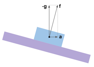
In the comments to the post about the filter Majvika flashed the question of whether it is possible to hope that this filter is less susceptible to acceleration than, for example, the Mahoney filter. Alas, all the filters described here exploit the same physical principles and therefore suffer from the same problems. To deceive physics by mathematics is impossible. What then to do?

The easiest and rough way was invented back in the middle of the last century for aviation gyroverticules: to reduce or completely zero the control angular velocity in the presence of accelerations or angular velocity of the course (which indicates the entrance to the turn). The same method can be transferred to the current freeware systems. Accelerations should be judged by the values.

$\hat{f}_{N}, \hat{f}_{E}$ , but not

$\hat{f}_{x}, \hat{f}_{y}$ which are in themselves a zero bend. However in magnitude

$\hat{\mathbf{f}}_{NED}$ it is not always possible to distinguish the true accelerations from the projections of the acceleration of gravity, thereby caused by the inclination of the gyro platform that needs to be eliminated. Therefore, the method does not work reliably - but does not require any additional sensors.

A more accurate method is based on using external velocity measurements from a GNSS receiver. If speed is known

$\mathbf{v}$ then it can be differentiated numerically and get true acceleration

$\dot{\mathbf{v}}$ . Then the difference

$\hat{\mathbf{f}}_{NED}-\dot{\mathbf{v}}$ will be exactly equal

$-\hat{\mathbf{g}}_{NED}$ regardless of carrier movement. It can be used as a standard of the vertical. For example, you can set the control angular velocity gyro in the form

$\omega'_{N}=gk_{g}(\hat{f}_{E}-\dot{v}_{E}),\; \omega'_{E}=-gk_{g}(\hat{f}_{N}-\dot{v}_{N})$

Sensor Zero Offsets

The sad feature of consumer-grade gyroscopes and accelerometers is the large volatility of zero offsets in time and temperature. To eliminate them, it is not enough to have only factory or laboratory calibration - you need to reassess during operation.

Gyroscopes. Understand the zero offsets of the gyros

$\delta{\mathbf{\omega}}$ . The calculated position of the associated coordinate system moves away from its true position with an angular velocity determined by two opposing factors — gyro zero shifts and an angular velocity control:

$\delta{\mathbf{\omega}}-\mathbf{\omega'}$ . If the correction system (for example, in the Mahoney filter) succeeded in stopping the care, then in the steady state it will be

$\delta{\mathbf{\omega}}=\mathbf{\omega'}$ . In other words, in the control angular velocity

$\mathbf{\omega'}$ enclosed information about an unknown active disturbance

$\delta{\mathbf{\omega}}$ . Therefore, compensatory estimation can be applied : we do not know the magnitude of the perturbation directly, but we know what kind of corrective action is necessary in order to balance it. The estimation of gyro zero shifts is based on this. For example, in Mahoney, the estimate is updated by law

$\dot{\hat{\delta\mathbf{\omega}}}=k_{b}\mathbf{\omega'}$

However, the result he gets is strange: the estimates reach 0.04 rad / s. Even the nastiest gyros do not have this instability of zero offsets. I suspect the problem is that Mahoney does not use GNSS or other external sensors - and is fully affected by the effects of accelerations. Only on the vertical axis, where accelerations do not harm, does the assessment look more or less robust:

Mahony et al., 2008

Accelerometers. Rate accelerometer zero offset

$\delta{\mathbf{f}}$ much harder. Information about them has to be extracted from the same control angular velocity.

$\mathbf{\omega'}$ . However, in the rectilinear motion, the effect of zero displacement of accelerometers is indistinguishable from the slope of the carrier or the skewing of the installation of the sensor unit on it. No addition to

$\mathbf{\omega'}$ accelerometers do not create. The additive appears only at a turn, as allows to divide and independently estimate errors of gyroscopes and accelerometers. An example of how this can be done is in my article . Here are pictures from there:

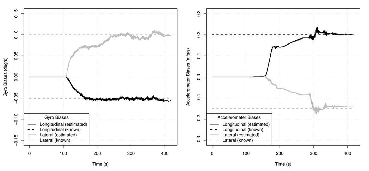
Instead of a conclusion: what about the Kalman filter?

I have no doubt that the filters described here will almost always have an advantage over the traditional Kalman filter in terms of speed, compactness of the code and convenience of customization - for this they were created. As for the accuracy of estimation, everything is not so clear. I met the unsuccessfully designed Kalman filters, which, in terms of accuracy, lost noticeably to the filter with the virtual gyroplatform. Madzhvik also argued the benefits of his filter with respect to some Kalman estimates. However, for the same orientation estimation task, at least a dozen different Kalman filter schemes can be constructed, and each will have an infinite number of tuning options. I have no reason to think that the Mahoney or Majvik filter will be more accurate than the best possibleKalman filters. And of course, the Kalman approach will always remain the advantage of universality: it does not impose any rigid restrictions on the specific dynamic properties of the system being evaluated.

Tags: