Reduction of neural networks using variational optimization
Hi, Habr. Today I would like to develop the topic of variation optimization and tell you how to apply it to the task of cropping non-informative channels in neural networks (pruning). With it, you can relatively simply increase the "rate of fire" of the neural network, not perelopachivaya its architecture.

The idea of reducing unnecessary elements in machine learning algorithms is not at all new. In fact, it is older than the concept of deep learning: it was only earlier that the branches of the decisive trees were cut, and now the weights in the neural network.
The basic idea is simple: we find a subset of useless weights in the network and reset them. Without complete enumeration, it is difficult to say which weights really participate in the prediction, and which only pretend, but this is not required. Various regularization methods, Optimal Brain Damage and other algorithms work well. Why even remove any weight? It turns out that this improves the generalizing ability of the network: as a rule, insignificant weights either simply introduce noise into the prediction, or are specifically sharpened on the signs of a training dataset (ie, retraining artifact). In this sense, the reduction of connections can be compared with the method of disconnecting random neurons (dropout) during network training. In addition, if there are a lot of zeros in the network, it takes up less space in the archive and is able to reckon faster on some architectures.
It sounds good, but it is much more interesting to throw out not individual weights, but neurons from fully connected layers or channels from the bundles entirely. In this case, the effect of network compression and acceleration of predictions is observed much more clearly. But this is more complicated than the destruction of individual scales: if you try to carry out Optimal Brain Damage, taking the whole bundle instead of one connection, the results will most likely not be very impressive. In order to be able to remove a neuron without serious consequences, you need to specifically make sure that it does not have a single useful connection. For this you need to somehow encourage the "strong" neurons to become stronger, and the "weak" - weaker. This task is already familiar to us: in fact, we force the network to be sparsity inducing, with some restrictions on the grouping of weights.
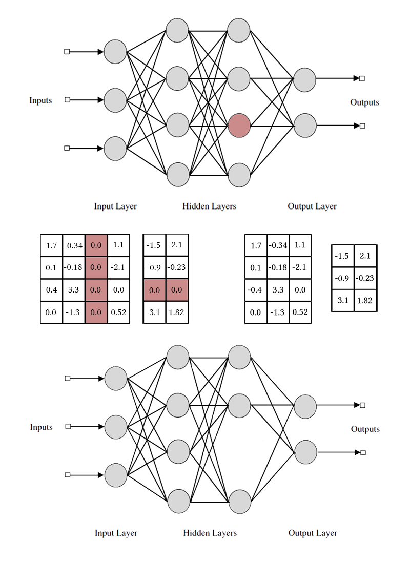
Note that in order to remove a single neuron or a convolutional channel, you need to modify two weight matrices. I will not make a distinction between convolutional channels and neurons: working with them is the same, only the specific weights that can be removed and the transposition method differ.
To begin with, let me tell you about the simplest and most effective way of removing extra neurons from the network - group LASSO regularization. Most often, it is used to keep useless weights in networks close to zero; it is trivially generalized to the case-by-channel case. Unlike regular regularization, we do not regularize weights or activate the layer directly, the idea is a little trickier. [Channel Pruning for Accelerating Very Deep Neural Networks; Yihui He et al; 2017]
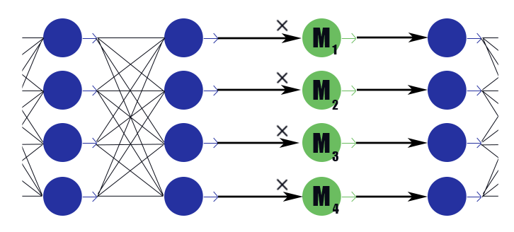
Consider a special masking layer with a weight vector . His conclusion is simply the work of elements.
 on the conclusions of the previous layer, it does not have an activation function. We will place on the masking layer after each layer, the channels in which we want to discard, and expose the weights in these layers to L1 regularization. Thus the weight of the mask
 multiplying by the ith output of the layer implicitly imposes a limit on all the weights on which this output depends. If among these scales, say half the useful, then
 will keep closer to one, and this output will be able to convey information well. But if only one or none at all,will drop to zero, which will nullify the output of the neuron and, in fact, will nullify all the weights on which this conclusion depends (in the case of an activation function equal to zero at zero). Note that this way the network receives less negative reinforcement in the case of legally large weights, or a legitimate strong response. Matters the utility of the neuron as a whole.
It turns out this formula:
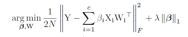
Where - the weighting constant of the loss of the network and the loss of rarefaction. It looks like the usual L1-regularization formula, only the second term contains vectors of masking layers, and not network weights.
After completing the training of the network, we run over neurons and masking their values. If a greater than a certain threshold, the neuron weights are multiplied by , if it is less, then the elements corresponding to the neuron are removed from the matrices of incoming and outgoing weights (as in the picture a little higher). After this, the masks can be dropped and completed the network.
In the application of group LASSO there are several subtleties:
But we are not looking for easy ways, right?
Channel rejection using L1 regularization is not entirely fair. It allows the channel to move along the “strong response” - “weak response” - “zero response” scale. Only when the masking weight is close enough to zero, we discard the channel using the capture mask. Such a movement distorts the picture nicely and makes changes to other channels during training: before they can learn what to do when the previous neuron is completely disconnected, they must learn what to do when it systematically gives a weak response.
Let me remind you that, ideally, we would like to greedily choose the least informative channel from the network, continue learning the network without it, remove the next least informative channel, adjust the network again, and so on. Alas, in this formulation, the problem is computationally unaffordable even for relatively simple networks. In addition, this approach does not leave the channels of a second chance - once removed, the neuron can not return to the system again. Let's slightly change the task: we will sometimes delete a neuron, and sometimes leave. Moreover, if the neuron is generally useful, leave it more often, and if it is useless, it is the other way around. For this, we will use the same masking layers as in the case of L1-regularization (it was not for nothing that they were introduced!). Only their weights will not move along the entire real axis with the attractor at zero, but will be concentrated around 0 and 1. Not that it becomes much simpler,
The instinct of the network educator suggests that you should not solve the problem of brute force, but you need to add the number of active neurons in layers on the current run to the loss function. However, such a member in loss will be stepwise constant, and the gradient descent will not be able to work with it. It is necessary to somehow teach the learning algorithm to periodically exclude some neurons, despite the absence of a gradient.
We have a way to temporarily remove neurons: we can apply a dropout to the masking layer. Let during training with probability
  and
and  with probability
  . Now you can put the sum in the loss functionwhich is a valid number. Here we are faced with another obstacle: the distribution is discrete, it is not clear how to work with it backpropagation'u. In general, there are special optimization algorithms that can help us here (see REINFORCE), but we will take a different approach.
It was then that the moment came where variational optimization comes into play : we can bring the discrete distribution of zeros and ones in the masking layer up to continuous and optimize the parameters of the latter using the usual back-propagation algorithm. This is the idea behind the work [Learning Sparse Neural Networks Through L0 Regularization; Christos Louizos et al; 2017].
The role of continuous distribution will be played by hard concrete distribution [The Concrete Distribution: A Continuous Relaxation of Discrete Random Variables; Chris Maddison; 2017], this is such a tricky logarithm piece, approximating the Bernoulli distribution:
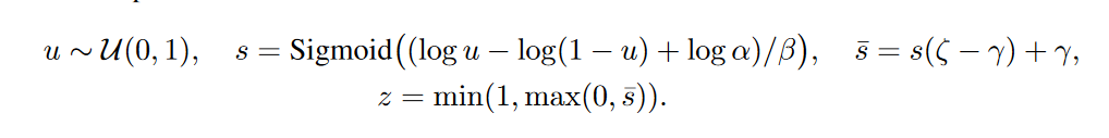
 - offset distribution relative to the center, and
  - temperature. With
 distribution is increasingly beginning to approximate the true Bernoulli distribution, but is losing differentiability. With
 distribution density is concave (this is the case of interest), with
  - is convex. We skip this distribution through a rigid sigmoid so that it can skillfully issue a finite non-zero probability.
 and
and  , and on the interval (0, 1) it had a continuous differentiable density. After the end of pruning, we look in which direction the distribution has shifted and replace the random variable
 to a specific mask value and bring to a condition already deterministic model.
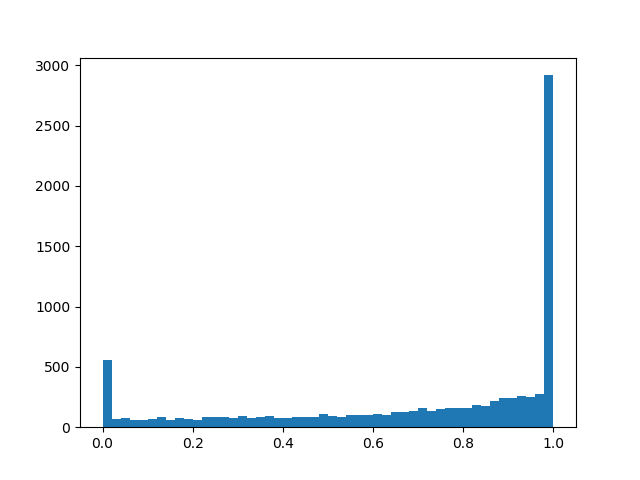
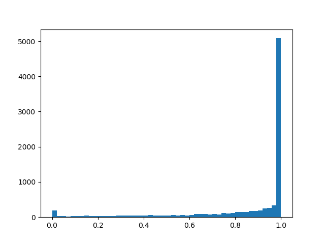
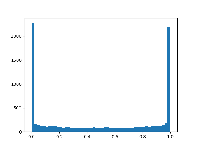
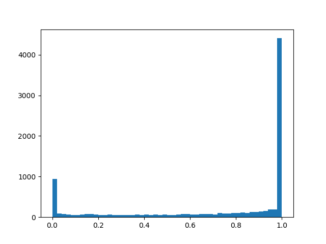
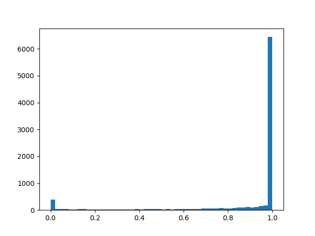
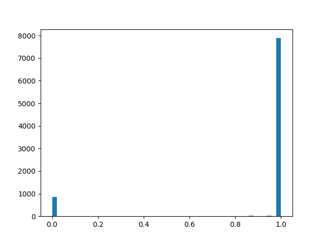
To feel a little better distribution, I will give several examples of its density for different parameters:
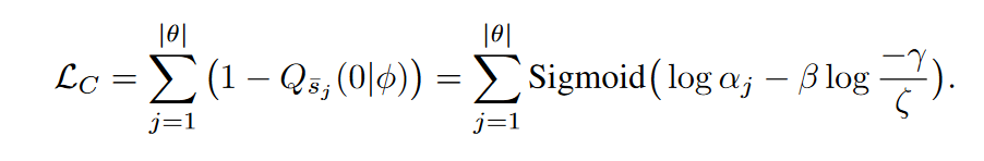
In fact, we have a “smart” dropout layer that learns which conclusions to throw more often. But what exactly are we optimizing? The loss should be placed integral of the distribution density in a non-zero region (the probability that the mask will be equal to non-zero during training is more simple):
The following features are added to the push-pull training, regular regularization and other implementation details mentioned in the L1 regularization chapter:
For the experiment, we take the CIFAR-10 dataset and a relatively simple network in four convolutional layers, followed by two fully connected ones: Conv2D, Mask, Conv2D, Mask, Pool2D, Conv2D, Mask, Conv2D, Mask, Pool2D, Flatten, Dropout (p = 0.5) , Dense, Mask, Dense (logits). It is believed that the pruning algorithms work better on thicker networks, but here I am faced with a purely technical problem of lack of computing power. Adam with learning rate = 0.0015 and batch size = 32 was used as an optimizer. In addition, the usual L1 (0.00005) and L2 (0.00025) regularizations were used. Image augmentation was not applied. The network studied 200 epochs before convergence, after which it was preserved, and neuron reduction algorithms were applied to it.
In addition to using the algorithms described above for pruning, we set a trivial reading point to make sure that the algorithms do something at all. Let's try alternately throwing out of each layer first neurons and retrain the resulting network.
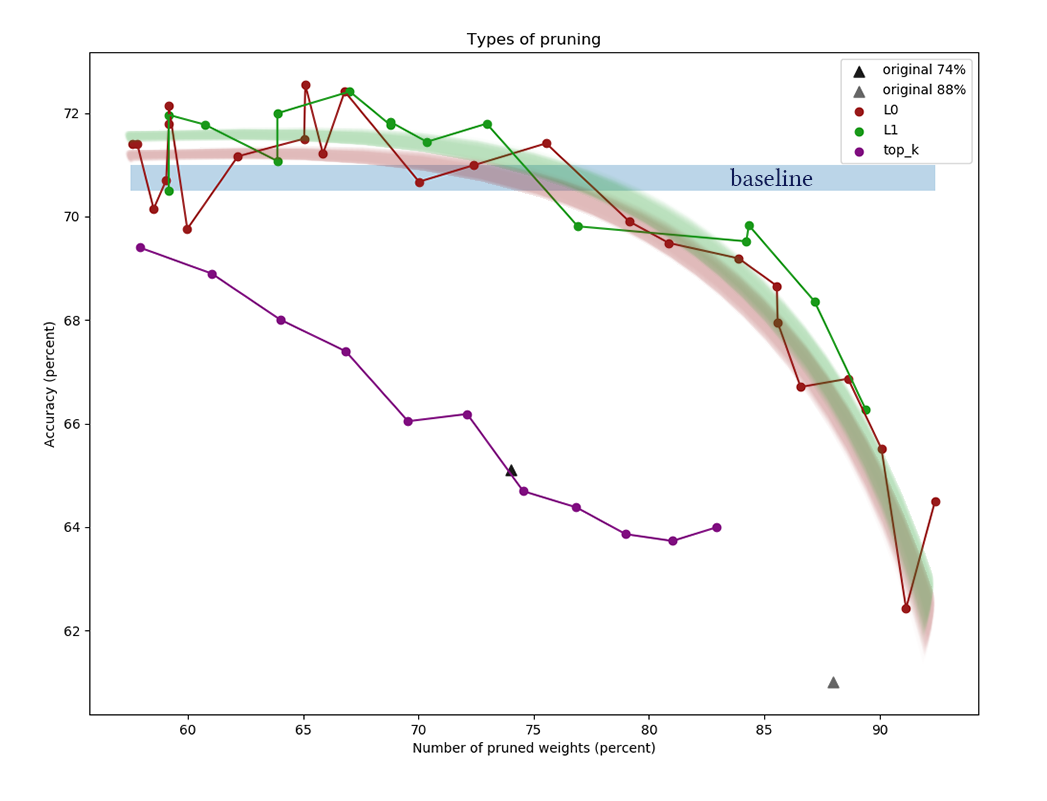
The graph shows the results of comparing L1 and L0 channel reduction algorithms after a series of experiments with different regularization power constants. On the X axis, the decrease in the number of weights in percent after the application of the algorithm is postponed . Y-axis - accuracy of the cut network on the validation sample. The blue bar in the middle is the approximate quality of the network, which has not yet been cut by neurons. The green line represents a simple L1 mask learning algorithm. The red line is L0-pruning. Purple line - delete firstchannels. Black triangles - learning network, which initially had a smaller number of scales.
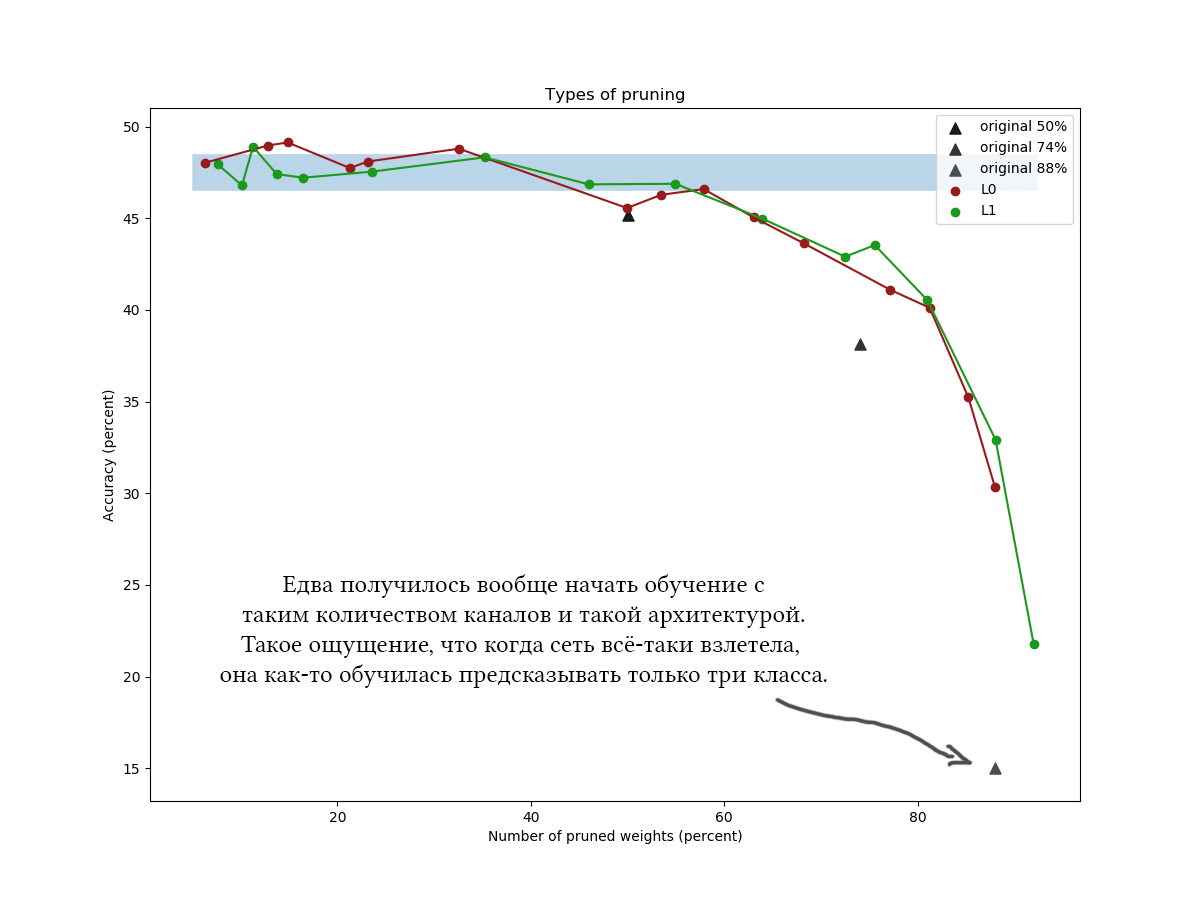
Another example for CIFAR-100 and a slightly longer and wider network is about the same architecture and with similar learning parameters:
Iiii on the graphs clearly show that a simple L1 algorithm copes just as well as clever variational optimization, and as if even a little more improves the quality of the network at low values of compression. The results are also confirmed by one-time experiments with other datasets and network architectures. This is an absolutely expected result, which I hoped for when I began experiments on the reduction of networks. Fair. Sigh.
Well, to be honest, I was a little surprised and tried to play with the algorithm and the network: different architectures, hyper parameters of the network, exact formulas of hard concrete distribution, initial values and , the number of epochs of intermediate adjustment. L0-regularization looks cool in theory, but in practice it is more difficult for it to choose hyper parameters, and it is considered longer, so I would not advise using it without additional experiments and file processing. Please do not consider the time spent reading the article: L0-pruning looks really very plausible, and I would say that rather, I somewhere incorrectly applied an algorithm that I did not receive the promised increase. Plus, variational optimization is the basis for even more advanced reduction algorithms [for example, Compressing Neural Networks using the Variational
Information Bottleneck, 2018].
In general, the following conclusions can be drawn:
Remember, as I wrote at the beginning of the post, that after the completion of the pruning algorithm, you can “just cut out unnecessary pieces of the network entirely”? So, cut the extra pieces of the network is not easy. Tensorflow and other libraries build a computational graph, and it cannot be so easily changed when it is already in operation. You have to save the network with the calculated masks, rip out the list of necessary weights from it, transpose the weights as necessary, delete the zeroed groups, transpose back, and create a new network based on the output set of tensors. The resulting network should have the same layout as the original, but it will have fewer neurons. Expect a headache with maintaining the same network scheme in the function of creating the initial and final network, especially if they are not linear, but branchy.
Probably for convenient masking you will have to create your own layers. This is easy, but be careful what collections you add masking options to. It is easy to make a mistake and accidentally train the parameters of the reduction of the channels along with all the other weights.
It should be noted that a significant part of the weights of networks with not very deep architectures is usually concentrated on the transition from the convolutional part to the fully connected. This is due to the fact that the last convolutional layer is made flat, as a result of which (the number of channels) * (width) * (height) of neurons are formed in it, and the next weights matrix is very wide. These weights are unlikely to cut; moreover, this should not be done, otherwise the last layers of the network will turn out to be “blind” to features found in some places. Try in such cases to make the final number of channels smaller and use maxpool'ingom or even use fully convolutional or fully fully connected architectures.
Thank you all for your attention, if it is interesting for someone to repeat the experiments on CIFAR-10 and CIFAR-100,The code can be taken on a githaba . Good working day!
The idea of reducing unnecessary elements in machine learning algorithms is not at all new. In fact, it is older than the concept of deep learning: it was only earlier that the branches of the decisive trees were cut, and now the weights in the neural network.
The basic idea is simple: we find a subset of useless weights in the network and reset them. Without complete enumeration, it is difficult to say which weights really participate in the prediction, and which only pretend, but this is not required. Various regularization methods, Optimal Brain Damage and other algorithms work well. Why even remove any weight? It turns out that this improves the generalizing ability of the network: as a rule, insignificant weights either simply introduce noise into the prediction, or are specifically sharpened on the signs of a training dataset (ie, retraining artifact). In this sense, the reduction of connections can be compared with the method of disconnecting random neurons (dropout) during network training. In addition, if there are a lot of zeros in the network, it takes up less space in the archive and is able to reckon faster on some architectures.
It sounds good, but it is much more interesting to throw out not individual weights, but neurons from fully connected layers or channels from the bundles entirely. In this case, the effect of network compression and acceleration of predictions is observed much more clearly. But this is more complicated than the destruction of individual scales: if you try to carry out Optimal Brain Damage, taking the whole bundle instead of one connection, the results will most likely not be very impressive. In order to be able to remove a neuron without serious consequences, you need to specifically make sure that it does not have a single useful connection. For this you need to somehow encourage the "strong" neurons to become stronger, and the "weak" - weaker. This task is already familiar to us: in fact, we force the network to be sparsity inducing, with some restrictions on the grouping of weights.
Note that in order to remove a single neuron or a convolutional channel, you need to modify two weight matrices. I will not make a distinction between convolutional channels and neurons: working with them is the same, only the specific weights that can be removed and the transposition method differ.
Easy way: group L1 regularization
To begin with, let me tell you about the simplest and most effective way of removing extra neurons from the network - group LASSO regularization. Most often, it is used to keep useless weights in networks close to zero; it is trivially generalized to the case-by-channel case. Unlike regular regularization, we do not regularize weights or activate the layer directly, the idea is a little trickier. [Channel Pruning for Accelerating Very Deep Neural Networks; Yihui He et al; 2017]
Consider a special masking layer with a weight vector
. His conclusion is simply the work of elements.on the conclusions of the previous layer, it does not have an activation function. We will place on the masking layer after each layer, the channels in which we want to discard, and expose the weights in these layers to L1 regularization. Thus the weight of the maskmultiplying by the ith output of the layer implicitly imposes a limit on all the weights on which this output depends. If among these scales, say half the useful, thenwill keep closer to one, and this output will be able to convey information well. But if only one or none at all,will drop to zero, which will nullify the output of the neuron and, in fact, will nullify all the weights on which this conclusion depends (in the case of an activation function equal to zero at zero). Note that this way the network receives less negative reinforcement in the case of legally large weights, or a legitimate strong response. Matters the utility of the neuron as a whole. It turns out this formula:
Where
- the weighting constant of the loss of the network and the loss of rarefaction. It looks like the usual L1-regularization formula, only the second term contains vectors of masking layers, and not network weights. After completing the training of the network, we run over neurons and masking their values. If a
greater than a certain threshold, the neuron weights are multiplied by , if it is less, then the elements corresponding to the neuron are removed from the matrices of incoming and outgoing weights (as in the picture a little higher). After this, the masks can be dropped and completed the network. In the application of group LASSO there are several subtleties:
- Regular regularization. Coupled with the regularization of masking weights, L1 / L2 regularization should be applied to all other weights of the network. Without this, a decrease in the masking weight in the case of unsaturated activation functions (ReLu, ELu) will easily be compensated for by an increase in weights, and the nulling effect will not work. Yes, and for ordinary sigmoid it allows you to better start the process with positive feedback:
 uninformative output becomes smaller, because of what the optimizer has to think more about each specific weight, because of what the output becomes even more uninformative, because of what decreases even more and so on.
 - The authors of the article also advise to impose a spherical limit on the weights of the layers.
 . Probably, this should contribute to the “flow” of weights from weak neurons to strong ones, but I did not notice much difference.
 - Push-pull training. The authors of the article suggest alternately training the usual neural network weights and masking weights. It's longer than teaching everything at once, but what about the results a little better?
- Do not forget about the long-term fine tuning of the network (fine-tuning) after fixing the mask, this is very important.
- Watch carefully how your masks stand: before or after the activation function. You may have activation issues that are not zero with an argument of zero (for example, sigmoid).
- Pruning is not friendly with batchnorm for about the same reason why dropout is not friendly with it: from the point of view of normalization, when in a bundle 32 values of which 12 are zero, and when in a bundle 20 values are very different situations. After the zeroing of the scales, the distribution learned by the batchnorm layer ceases to be valid. It is necessary either to insert pruning layers after all batchnorm layers, or to somehow modify the latter.
- There are also difficulties with the application of channel reduction to "branchy" architectures and residual-networks (ResNet). After cutting off extra neurons during the merging of branches, the dimensions may not coincide. This is easily solved by the introduction of buffer layers, in which we do not reject neurons. In addition, if the network branches carry different amounts of information, it makes sense to set different for themso that it doesn't turn out that Pruning simply cut all the neurons in the least informative branch. However, if all the neurons cut, then the branch is not so important?
- In the original formulation of the problem there is a hard limit on the number of non-zero channels, but in my opinion, it suffices to change only the weighting parameter of the initial loss and L1-loss of masking weights, and then let the optimizer decide how many channels to leave.
- Masks capture. This is not in the original article, but in my opinion, this is a good practical mechanism for improving convergence. When the mask value reaches a predetermined low value, we reset it and prohibit changing this part of the mask. Thus, the weak weights completely stop contributing to the prediction already during the training of the model, and do not add any parasitic values to the corresponding amounts. Theoretically, this could prevent a potentially useful channel from returning to service, but I do not think that this happens in practice.
Difficult way: L0-regularization
But we are not looking for easy ways, right?
Channel rejection using L1 regularization is not entirely fair. It allows the channel to move along the “strong response” - “weak response” - “zero response” scale. Only when the masking weight is close enough to zero, we discard the channel using the capture mask. Such a movement distorts the picture nicely and makes changes to other channels during training: before they can learn what to do when the previous neuron is completely disconnected, they must learn what to do when it systematically gives a weak response.
Let me remind you that, ideally, we would like to greedily choose the least informative channel from the network, continue learning the network without it, remove the next least informative channel, adjust the network again, and so on. Alas, in this formulation, the problem is computationally unaffordable even for relatively simple networks. In addition, this approach does not leave the channels of a second chance - once removed, the neuron can not return to the system again. Let's slightly change the task: we will sometimes delete a neuron, and sometimes leave. Moreover, if the neuron is generally useful, leave it more often, and if it is useless, it is the other way around. For this, we will use the same masking layers as in the case of L1-regularization (it was not for nothing that they were introduced!). Only their weights will not move along the entire real axis with the attractor at zero, but will be concentrated around 0 and 1. Not that it becomes much simpler,
The instinct of the network educator suggests that you should not solve the problem of brute force, but you need to add the number of active neurons in layers on the current run to the loss function. However, such a member in loss will be stepwise constant, and the gradient descent will not be able to work with it. It is necessary to somehow teach the learning algorithm to periodically exclude some neurons, despite the absence of a gradient.
We have a way to temporarily remove neurons: we can apply a dropout to the masking layer. Let during training
with probability and with probability . Now you can put the sum in the loss functionwhich is a valid number. Here we are faced with another obstacle: the distribution is discrete, it is not clear how to work with it backpropagation'u. In general, there are special optimization algorithms that can help us here (see REINFORCE), but we will take a different approach. It was then that the moment came where variational optimization comes into play : we can bring the discrete distribution of zeros and ones in the masking layer up to continuous and optimize the parameters of the latter using the usual back-propagation algorithm. This is the idea behind the work [Learning Sparse Neural Networks Through L0 Regularization; Christos Louizos et al; 2017].
The role of continuous distribution will be played by hard concrete distribution [The Concrete Distribution: A Continuous Relaxation of Discrete Random Variables; Chris Maddison; 2017], this is such a tricky logarithm piece, approximating the Bernoulli distribution:
- offset distribution relative to the center, and - temperature. Withdistribution is increasingly beginning to approximate the true Bernoulli distribution, but is losing differentiability. With distribution density is concave (this is the case of interest), with - is convex. We skip this distribution through a rigid sigmoid so that it can skillfully issue a finite non-zero probability. and , and on the interval (0, 1) it had a continuous differentiable density. After the end of pruning, we look in which direction the distribution has shifted and replace the random variable to a specific mask value and bring to a condition already deterministic model. To feel a little better distribution, I will give several examples of its density for different parameters:
Distribution density :
:
 :
:
 :
:
 :
:
 :
:
 :
:
 :
:
 :
:
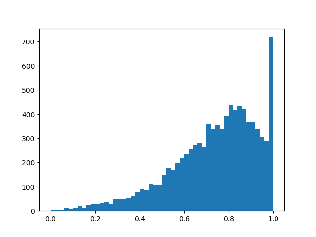
: : : : : : : : In fact, we have a “smart” dropout layer that learns which conclusions to throw more often. But what exactly are we optimizing? The loss should be placed integral of the distribution density in a non-zero region (the probability that the mask will be equal to non-zero during training is more simple):
The following features are added to the push-pull training, regular regularization and other implementation details mentioned in the L1 regularization chapter:
- Once again: our “smart” th dropout-layer with a noticeable probability resets the output, with a certain - it leaves it as it is, and plus, there is a small chance depending on
 that the output will be multiplied by a random number from 0 to 1. The last part is more parasitic than useful for our final goal, but without it in any way - it is needed for the back passage backpropagation'a.
 - General and and - trained parameters, but in my experiments I felt that if you just set a small (0.05) and in the process of learning it is still linearly reduced, the algorithm converges better than if it is honestly learned. better set big enough
 so that the neurons were initially preserved more often than they were discarded, but not large enough for the sigmoid to be saturated with loss.
 - If replaced in the formulas
 on just as if the network converges better and is less likely to run into NaN during training. With this maneuver, you need to remember to change the term in the function of losses and initialization.
 - Also, if you cheat and replace the usual sigmoid in loss with a hard one with restrictions on
![$ \ log {\ alpha} \ in [-4, 4] $](https://habrastorage.org/getpro/habr/formulas/3cd/5cf/6e4/3cd5cf6e4289463f9460e9e8dad37218.svg) , regularization will better converge and act stronger.
, regularization will better converge and act stronger. - TO and You can additionally apply regularization to further increase sparseness.
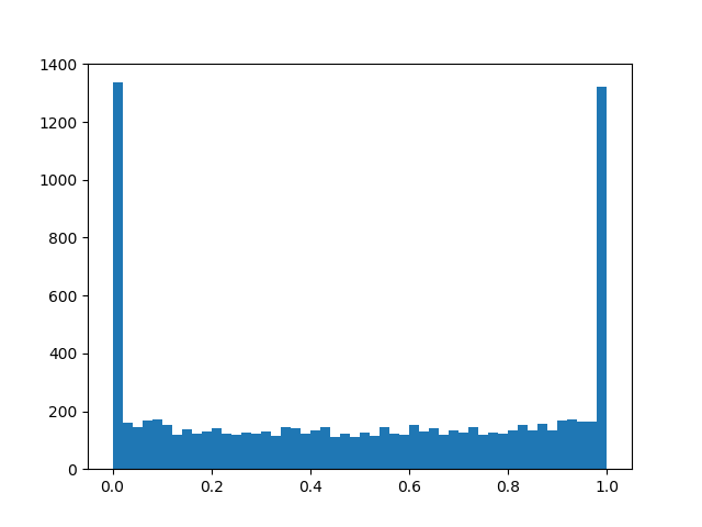
- After the end of the training session, one should binarize the results obtained and persistently train the network with a deterministic mask until val accuracy is released to a constant. The article provides a more accurate formula by which the output of a neuron can be made deterministic during validation or for the release of a network, but it seems that by the end of training turn out to be sufficiently polarized for simple heuristics to work:
 - mask 0,
  - mask 1 (but this is not accurate). After the transition to deterministic masks you will see a jump in quality. Do not forget that we came here to reset the weight, and below a certain weight threshold, you still need to replace the masking weights with zeros.
 - An additional plus of the L0 approach is that the masking layers start working as a dropout, which brings a powerful regularizing effect to the network. But this is a double-edged sword: if you start learning with too little, there is a risk of destroying a pre-trained network structure.
Experiments
For the experiment, we take the CIFAR-10 dataset and a relatively simple network in four convolutional layers, followed by two fully connected ones: Conv2D, Mask, Conv2D, Mask, Pool2D, Conv2D, Mask, Conv2D, Mask, Pool2D, Flatten, Dropout (p = 0.5) , Dense, Mask, Dense (logits). It is believed that the pruning algorithms work better on thicker networks, but here I am faced with a purely technical problem of lack of computing power. Adam with learning rate = 0.0015 and batch size = 32 was used as an optimizer. In addition, the usual L1 (0.00005) and L2 (0.00025) regularizations were used. Image augmentation was not applied. The network studied 200 epochs before convergence, after which it was preserved, and neuron reduction algorithms were applied to it.
In addition to using the algorithms described above for pruning, we set a trivial reading point to make sure that the algorithms do something at all. Let's try alternately throwing out of each layer first
neurons and retrain the resulting network. The graph shows the results of comparing L1 and L0 channel reduction algorithms after a series of experiments with different regularization power constants. On the X axis, the decrease in the number of weights in percent after the application of the algorithm is postponed . Y-axis - accuracy of the cut network on the validation sample. The blue bar in the middle is the approximate quality of the network, which has not yet been cut by neurons. The green line represents a simple L1 mask learning algorithm. The red line is L0-pruning. Purple line - delete first
channels. Black triangles - learning network, which initially had a smaller number of scales. Another example for CIFAR-100 and a slightly longer and wider network is about the same architecture and with similar learning parameters:
Iiii on the graphs clearly show that a simple L1 algorithm copes just as well as clever variational optimization, and as if even a little more improves the quality of the network at low values of compression. The results are also confirmed by one-time experiments with other datasets and network architectures. This is an absolutely expected result, which I hoped for when I began experiments on the reduction of networks. Fair. Sigh.
Well, to be honest, I was a little surprised and tried to play with the algorithm and the network: different architectures, hyper parameters of the network, exact formulas of hard concrete distribution, initial values
and , the number of epochs of intermediate adjustment. L0-regularization looks cool in theory, but in practice it is more difficult for it to choose hyper parameters, and it is considered longer, so I would not advise using it without additional experiments and file processing. Please do not consider the time spent reading the article: L0-pruning looks really very plausible, and I would say that rather, I somewhere incorrectly applied an algorithm that I did not receive the promised increase. Plus, variational optimization is the basis for even more advanced reduction algorithms [for example, Compressing Neural Networks using the Variational Information Bottleneck, 2018].
In general, the following conclusions can be drawn:
- Many channels in a trained network are clearly redundant. Even when setting a small regularization mask constant, it is easy to achieve a reduction of 30-50% of the weights. But if you initially train too “thin” mesh, it is difficult to achieve good results. This speaks in favor of the beneficial effects of the broad strata on the target network function and in favor of the lottery ticket theory [The Lottery Ticket Hypothesis: Training Pruned Neural Networks, J. Frankle and M. Carbin, 2018] (the more neurons, the more likely that one of them would be initialized so that it would form a good rule).
- If you start with a wide network and gradually throw out channels with additional training, then the network keeps quite well. But if you immediately throw out too many scales without completing the training, the accuracy of the network will irreparably deteriorate. Is the plasticity of neurons better performing when the network is close to the optimal state?
- Although it is impossible to reduce the number of scales for an arbitrarily long time, in this matter one can go surprisingly far. Judging by the scientific articles and my experiments, the decline usually begins in the region of 60-90% compression by weights. Although in my experiments the gap between the curves of the algorithms for the reduction of neurons and the ejection curves of the first neurons accounted for <7%, many scientific articles report a much greater superiority.
- Please note that in the case of weak compression (<60%), neuron reduction algorithms work as regularizers: the accuracy on the validation sample after the operation of the algorithms is even higher than the original!
- In addition to L1 and L0, channel trimming algorithms were tried by the magnitude of the weights and the average number of zeros of the activation function (APoZ), but they are not represented on the graph, since proved to be barely better than just zeroing the top channels.
- In articles, they usually train the network until it stops, and only then apply to it the algorithms for cutting off extra neurons. This is done, as I understand it, for the purity of the experiment, and so that it can be seen that the quality of the network slightly deteriorated relative to the reference point. But if you already know the architecture and the basic accuracy with which you are competing, then preliminary training before reaching the bar seems to be optional. Anyway, after the start of the pruning algorithm, the weights are very cool perekolbashivayutsya, and initially the accuracy drops significantly. You can train the network to a more or less sane state, and then simultaneously train and clean the network.
A few words about the technical side of the issue
Remember, as I wrote at the beginning of the post, that after the completion of the pruning algorithm, you can “just cut out unnecessary pieces of the network entirely”? So, cut the extra pieces of the network is not easy. Tensorflow and other libraries build a computational graph, and it cannot be so easily changed when it is already in operation. You have to save the network with the calculated masks, rip out the list of necessary weights from it, transpose the weights as necessary, delete the zeroed groups, transpose back, and create a new network based on the output set of tensors. The resulting network should have the same layout as the original, but it will have fewer neurons. Expect a headache with maintaining the same network scheme in the function of creating the initial and final network, especially if they are not linear, but branchy.
Probably for convenient masking you will have to create your own layers. This is easy, but be careful what collections you add masking options to. It is easy to make a mistake and accidentally train the parameters of the reduction of the channels along with all the other weights.
It should be noted that a significant part of the weights of networks with not very deep architectures is usually concentrated on the transition from the convolutional part to the fully connected. This is due to the fact that the last convolutional layer is made flat, as a result of which (the number of channels) * (width) * (height) of neurons are formed in it, and the next weights matrix is very wide. These weights are unlikely to cut; moreover, this should not be done, otherwise the last layers of the network will turn out to be “blind” to features found in some places. Try in such cases to make the final number of channels smaller and use maxpool'ingom or even use fully convolutional or fully fully connected architectures.
Thank you all for your attention, if it is interesting for someone to repeat the experiments on CIFAR-10 and CIFAR-100,The code can be taken on a githaba . Good working day!