Kaggle: Amazon from Space - tricks and hacks when training neural networks

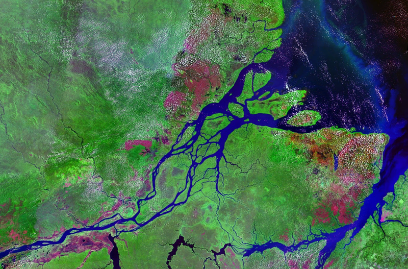
Last summer, the kaggle competition ended , which was devoted to the classification of satellite images of the Amazon forests. Our team took the 7th place from 900+ participants. Despite the fact that the competition has ended a long time ago, almost all the techniques of our solution are still applicable, and not only for competitions, but also for training neural networks for sale. For details under the cat.

tldr.py

import kaggle
from ods import albu, alno, kostia, n01z3, nizhib, romul, ternaus
from dataset import x_train, y_train, x_test
oof_train, oof_test = [], []
for member in [albu, alno, kostia, n01z3, nizhib, romul, ternaus]:
   for model in member.models:
       model.fit_10folds(x_train, y_train, config=member.fit_config)
       oof_train.append(model.predict_oof_tta(x_train, config=member.tta_config))
       oof_test.append(model.predict_oof_tta(x_test, config=member.tta_config))
for model in albu.second_level:
   model.fit(oof_train)
   y_test = model.predict_proba(oof_test)
y_test = kostia.bayes_f2_opt(y_test)
kaggle.submit(y_test)

Task Description

Planet has prepared a set of satellite images in two formats:

1. TIF - 16 bit RGB + N, where N is Near Infra Red
2. JPG - 8bit RGB, which are derived from TIF and that were provided to reduce the threshold for entering the task, as well as to simplify visualization. In a previous Kaggle competition, it was necessary to work with multispectral images. non-visual, that is, infrared, as well as channels with a longer wavelength greatly improved the quality of the prediction, and both the network and unsupervised methods.

Geographically, data were taken from the territory of the Amazon Basin, and from the territories of Brazil, Peru, Uruguay, Colombia, Venezuela, Guyana, Bolivia and Ecuador, in which interesting surface areas were selected, images of which were offered to the participants.

After creating jpg from tif, all the scenes were cut into small pieces of size 256x256. And according to the received jpg, the Planet employees from the Berlin and San Francisco offices, as well as through the Crowd Flower platform, made the marking.

The participants were given the task to predict one of the mutually exclusive weather labels for each 256x256

tile : Cloudy, Partly cloudy, Haze, Clear

As well as 0 or more bad weather: Agriculture, Primary, Selective Logging, Habitation, Water, Roads, Shifting Cultivation, Blooming, Conventional Mining

Total 4 weather and 13 not weather, and the weather is mutually exclusive, and the weather is not, but if the label on the picture cloudy, then there should be no other tags.



The accuracy of the model was estimated by the F2 metric:

$$

$$

$$

$$

Moreover, all labels had the same weight and at first F2 was calculated for each picture, and then the total averaging was performed. Usually they do it a little differently, that is, a certain metric is calculated for each class, and then averaged. The logic is that the latter is more interpretable, since it allows you to answer the question of how the model behaves in each particular class. In this case, the organizers took the first option, which, apparently, is related to the specifics of their business.

Total in the train 40k samples. In the test 40k. Due to the small size of the dataset, but the large size of the pictures, it can be said that it is “MNIST on steroids”

Lyrical digression

As can be seen from the description, the task is quite clear and the solution is not rocket ideas: you just need to fix the grid. And taking into account the specifics of Kaggle, also a bunch of models on top. However, to get a gold medal, you must not just somehow train a bunch of models. It is extremely important to have a lot of basic various models, each of which in itself shows an outstanding result. And already on top of these models you can wind up stacking and other hacks.

member	net	1crop	Tta	diff,%
alno	densenet121	0.9278	0.9294	0.1736
nizhib	densenet169	0.9243	0.9277	0.3733
romul	vgg16	0.9266	0.9267	0.0186
ternaus	densenet121	0.9232	0.9241	0.0921
albu	densenet121	0.9294	0.9312	0.1933
kostia	resnet50	0.9262	0.9271	0.0907
n01z3	resnext50	0.9281	0.9298	0.1896

The table shows the F2 score models of all participants for single crop and TTA. As you can see, the difference is not great for real use, however it is important for the competition mode.

Team interaction

Alexander Buslaev albu
At the time of participation in the competition, he led all the mln direction in the company Geoscan. But since then he dragged a bunch of competitions, fathers became the whole ODS on semantic segmentation and went to Minsk, rowed to Mapbox, about which an article

Alexey Noskov alno came out .
Universal ml fighter. Worked at Evil Martians. Now rolled into Yandex.

Konstantin Lopukhin kostialopuhin
Worked and continues to work at Scrapinghub. Since then Kostya managed to get a few more medals and, without 5 minutes, Kaggle Grandmaster

Arthur Kuzin n01z3
At the time of participation in this competition, I was working in Avito. But around the new year, the start-up Dbrain rolled over to the Lead Data Scientist position in the blockchain . Hopefully, we will soon gladden the community with our contests with dockers and lamp markings.

Yevgeny Nizhibitsky @nizhib
Lead Data Scientist at Rambler & Co. From this competition, Zhenya discovered the secret ability to find faces in picture contests. What helped him to drag a couple of competitions on the Topcoder platform. I told about one of them .

Ruslan Baykulov romul
Engaged in tracking sports events in the company Constanta.

Vladimir Iglovikov ternaus You
could be remembered for an action-packed article about the oppression of British intelligence. He worked in TrueAccord, but then rolled into the trendy-youth Lyft. Where is Computer Vision for Self-Driving car. Continuing to haul the competition and recently received a Kaggle Grandmaster.

Our association and participation format can be called typical. The decision to unite was due to the fact that we all had close results on the leaderboard. And each of us sawed its own independent pipeline, which represented a completely autonomous solution from beginning to end. Also after the merger, several participants were engaged in stacking.

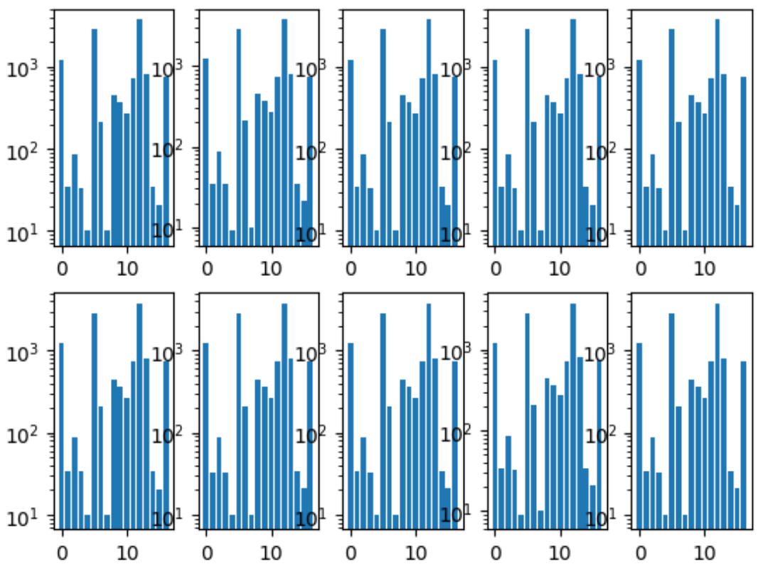
The first thing we did was general folds. We made it so that the distribution of classes in each fold was the same as in the entire dataset. To do this, they first selected the rarest class, stratified by it, because the remaining pictures were stratified according to the second most popular class, and so on until there are no pictures left.

Folder classes histogram:



We also had a common repository, where each team member had his own folder, within which he organized the code as he wanted.

And we also agreed on the format of the predicates, since this was the only point of interaction for combining our models.

Learning neural networks

As each of us had an independent pipeline, we were a gridsch of an optimal learning process parallel to people.

General approach


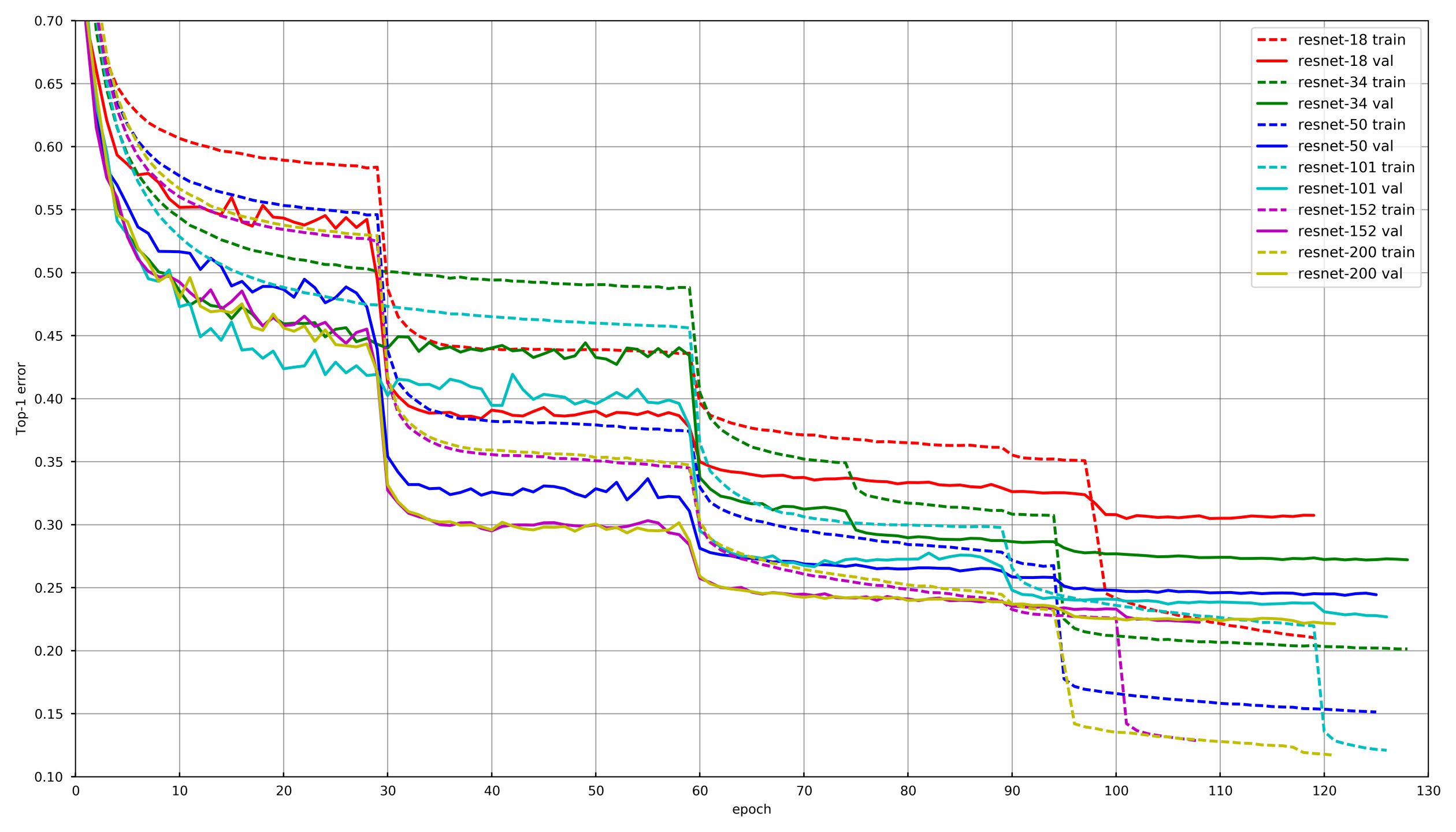
Picture from github.com/tornadomeet/ResNet

A typical learning process is presented on the Resnet neural networks training schedule on imagenet. Start with randomly initialized weights with SGD (lr 0.1 Nesterov Momentum 0.0001 WD 0.9) and then after 30 epochs lower the learning rate 10 times.

Conceptually, each of us used the same approach, but in order not to grow old while each network is being trained, the decrease in LR occurred if the validation loss did not fall 3-5 epochs in a row. Either some participants simply reduced the number of epochs at each LR damage and lowered them on a schedule.

Augmentations

Choosing the right augmentations is very important when training neural networks. Augmentation should reflect the variability of the nature of the data. Conventionally, augmentations can be divided into two types: those that introduce an offset to the data, and those that do not. Under the displacement can be understood various low-level statistics, such as histograms of colors or a characteristic size. In this regard, for example, HSV augmentation and scale - offset, but random crop - not.

In the early stages of network training, you can go overboard with augmentations and use a very hard set. However, towards the end of the training, you must either turn off the augmentations, or leave only those that do not contribute bias. This allows neural networks to overfit a little under the train and show a slightly better result on validation.

Freeze layers

In the overwhelming majority of tasks, it makes no sense to train a neural network from scratch; it is much more efficient to connect it from pre-trained networks, say, from Imagenet. However, you can go further and not just change the fully connected layer under the layer with the required number of classes, but train it first with freezing all the bundles. If you do not freeze convolutions and train the entire network at once with randomly initialized weights of the full mesh layer, then the weights of the convolutions are corrected and the final performance of the neural network will be lower. This task was especially noticeable due to the small size of the training sample. At other competitions with a large amount of data like cdiscount, it was possible to freeze not the entire neural network, but groups of bundles starting from the end. In this way, learning could be greatly accelerated, since gradients were not considered for the frozen layers.

Cyclic annealing

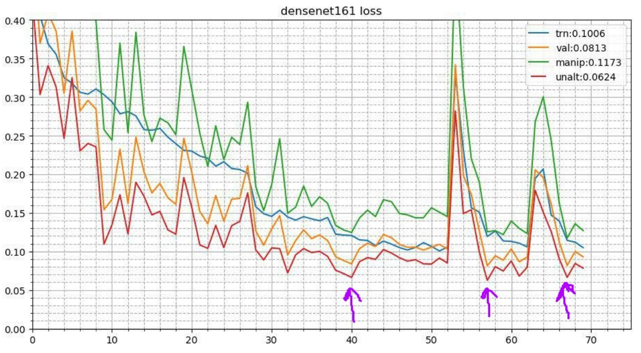
This process looks like this. After completing the basic learning process of the neural network, the best weights are taken and the learning process is repeated. But it starts from a lower learning rate and occurs in a short time, say 3-5 epochs. This allows the neural network to descend to a lower local minimum and show the best performance. This stable trip improves the result in a fairly wide range of contests.

In more detail about two receptions here

Test time augmentations

Since we are talking about competition and we have no formal limit on the time of inference, you can use augmentation during the test. It looks so that the picture is distorted as well as it happened during the training. Let's say it is reflected vertically, horizontally, rotated by an angle, etc. Each augmentation gives a new picture from which we get predictions. Then the predictions of such distortions of one picture are averaged (as a rule by the geometric average). It also gives a profit. In other contests, I also experimented with random home augmentation. Say, you can apply not one by one, but simply reduce the amplitude for random turns, contrasts and color augmentations by half, fix the seed and make several such randomly distorted images. This also gave an increase.

Snapshot Ensembling (Multicheckpoint TTA) The

idea of ​​annealing can be further developed. At each stage of annealing, the neural network flies into slightly different local minima. And this means that these are essentially slightly different models that can be averaged. Thus, during the predictions of the test, you can take the three best checkpoints and average their predictions. I also tried to take not the three best, but the three most diverse of the top 10 checkpoints - it was worse. Well, for production such a trick is not applicable and I tried to average the weights of the models. This gave a very small, but stable increase.



Approaches of each team member

Accordingly, to varying degrees, each member of our team used a different combination of the above techniques.

nick	Conv freeze, epoch	Optimizer	Strategy	Augs	Tta
albu	3	SGD	15 epoch LR decay, Circle 13 epochs	D4, Scale, Offset, Distortion, Contrast, Blur	D4
alno	3	SGD	Lr decay	D4, Scale, Offset, Distortion, Contrast, Blur, Shear, Channel multiplier	D4
n01z3	2	SGD	Drop LR, patient 10	D4, Scale, Distortion, Contrast, Blur	D4, 3 checkpoint
ternaus	-	Adam	Cyclic LR (1e-3: 1e-6)	D4, Scale, Channel add, Contrast	D4, random crop
nizhib	-	Adam	StepLR, 60 epochs, 20 per decay	D4, RandomSizedCrop	D4, 4 corners, center, scale
kostia	one	Adam		D4, Scale, Distortion, Contrast, Blur	D4
romul	-	SGD	base_lr: 0.01 - 0.02 lr = base_lr * (0.33 ** (epoch / 30)) Epoch: 50	D4, Scale	D4, Center crop, Corner crops

Stacking and Khaki

We trained each model with each set of parameters in 10 folds. And then on out of fold (OOF) predicates were taught models of the second level: Extra Trees, Linear Regression, Neural Network, and simply averaging the models.

And already on the OOF predicates of the models of the second level weighed the weights for mixing. You can read more about stacking here and here .

In real production, oddly enough, this approach also takes place. For example, when there are multi-modal data (pictures, text, categories, etc.) and I want to combine the predictions of models. You can simply average probabilities, but learning the second level model gives the best result.

Baes F2 Optimization

Also, the final predictions tyunilas a little using Bayes optimization. Suppose that we have ideal probabilities, then F2 with the best expectation mat (i.e. optimal type) is obtained according to the following formula:



What does this mean? It is necessary to go through all the combinations (i.e. for each label 0 and 1), calculate the probability of each combination, and multiply by F2 - we get the expected F2. For which combination it is better, and it will give the optimal F2. The probabilities were considered simply by multiplying the probabilities of the individual labels (if the label has 0, we take 1 - p), and not to go over 2 in 17 options, only labels with a probability from 0.05 to 0.5 wobbled - these were 3-7 in a row, so a little (submit was done in a couple of minutes). In theory, it would be cool to get the probability of a combination of labels not just by multiplying individual probabilities (because labels are not independent), but this is not the case.

what did it give? when the models became good, the selection of thresholds after the ensemble ceased to work, and this piece gave a small but stable gain both on validation and on public / private.

Afterword

As a result, we have trained 48 different models, each on 10 folds, i.e. 480 models of the first level. Such a human girdserch allowed me to try different techniques when learning deep convolutional neural networks, which I still use in work and competitions.

Was it possible to train fewer models and get the same or better result? Yes, it is quite. Our compatriots from the 3rd place Stanislav stasg7 Semenov and Roman ZFTurbo Solovyov managed a smaller number of first-level models and compensated for 250+ second-level models. Pro solution cansee the analysis and read the post.

First place went to the mysterious bestfitting. In general, this guy is very cool, and now he has become the top1 of the Kaggle rating, having dragged a lot of picture contests. He remained anonymous for a long time, until Nvidia tore off covers by interviewing him . In which he admitted that 200 subordinates would report to him ... There is also a post about the decision .

Another interesting fact : Jeremy Howard , widely known in narrow circles , fastai's father finished 22m. And if they thought that he had just sent a couple of submitters, they did not guess. He participated in the team and sent 111 parcels.

Also, graduate students at Stanford, who were passing the legendary CS231n course at that time, and who were allowed to use this task as a course project, ended up in the middle of a leaderboard with the whole team.

As a bonus, I spoke at Mail.ru with the material of this post and here is another presentation of Vladimir Iglovikov from the mitap in the Valley.