Improving image clarity based on frequency filtering in Matlab
Introduction
To date, many algorithms have been developed to improve the quality of images characterized by the speed of the complexity of mathematical methods, the requirements for the resources of a computer system, etc. Moreover, one of the simplest methods is image processing based on its filtering in the frequency and spatial domains.
Basic concepts
The basis of linear filtering in the frequency and spatial domains is the convolution theorem. In fact, the main idea of filtering in the frequency domain is to select an accessory filter function that modifies F (u, v) in a specific way.
For example, a filter having an accessory function that, being multiplied by the centered function F (u, v), attenuates the high-frequency components of F (u, v), and leaves the low-frequency components relatively unchanged and is called the low-pass filter.
Images and their transformations are automatically considered periodic if filtering is implemented based on a two-dimensional Fourier transform.
When convolving periodic functions, interference effects arise between adjacent periods if these periods are located close to the length of the nonzero parts of the functions. Such interference is usually called a return error or an overlap error, which can be suppressed by supplementing the functions with zeros as follows:
Suppose that the functions f (x, y) and h (x, y) have dimensions AB and C D. We form two extended functions, both having dimensions P and Q, by adding zeros to f and g.
P≥A + C + 1 and Q≥B + D + 1
We calculate the minimum even values of P and Q that satisfy these conditions.
We implement the above algorithm as a function.
The transfer function of the filter H (u, v) is multiplied by the real and imaginary parts of F (u, v). If the function H (u, v) was real, then the phase part of the product does not change, as can be seen from the phase equation, since when the real and imaginary parts of the complex number are multiplied by the same number, the phase angle does not change. Such filters are commonly called filters with a zero phase shift.
We generate a filter H in the frequency domain corresponding to the spatial Sobel filter, which improves the vertical edges of the image.
The following dftuv function creates a grid array that is used in calculating distances and other similar actions.
I will give an example of creating a function that forms a low-pass filter.
Now an example of creating a function forming a high-pass filter.
And the script itself to increase the clarity of images using the above functions.
**** Examples of work **** Final result

To date, many algorithms have been developed to improve the quality of images characterized by the speed of the complexity of mathematical methods, the requirements for the resources of a computer system, etc. Moreover, one of the simplest methods is image processing based on its filtering in the frequency and spatial domains.
Basic concepts
The basis of linear filtering in the frequency and spatial domains is the convolution theorem. In fact, the main idea of filtering in the frequency domain is to select an accessory filter function that modifies F (u, v) in a specific way.
For example, a filter having an accessory function that, being multiplied by the centered function F (u, v), attenuates the high-frequency components of F (u, v), and leaves the low-frequency components relatively unchanged and is called the low-pass filter.
Images and their transformations are automatically considered periodic if filtering is implemented based on a two-dimensional Fourier transform.
When convolving periodic functions, interference effects arise between adjacent periods if these periods are located close to the length of the nonzero parts of the functions. Such interference is usually called a return error or an overlap error, which can be suppressed by supplementing the functions with zeros as follows:
Suppose that the functions f (x, y) and h (x, y) have dimensions AB and C D. We form two extended functions, both having dimensions P and Q, by adding zeros to f and g.
P≥A + C + 1 and Q≥B + D + 1
We calculate the minimum even values of P and Q that satisfy these conditions.
We implement the above algorithm as a function.
- function PQ = paddedsize(AB, CD, PARAM)
- if nargin==1
- PQ=2*AB;
- elseif nargin == 2&~ischar(CD)
- PQ = AB+CD ;
- PQ= 2 *ceil (PQ/2);
- elseif nargin == 2
- m= max (AB);
- P=2^nextpow2(2*m);
- PQ=[P, P];
- elseif nargin==3
- m=max([AB CD]);
- P=2^nextpow2(2*m);
- PQ=[P, P];
- else
- error('Неправильные входные данные');
- end
- end
* This source code was highlighted with Source Code Highlighter.The transfer function of the filter H (u, v) is multiplied by the real and imaginary parts of F (u, v). If the function H (u, v) was real, then the phase part of the product does not change, as can be seen from the phase equation, since when the real and imaginary parts of the complex number are multiplied by the same number, the phase angle does not change. Such filters are commonly called filters with a zero phase shift.
- function g = dftfilt (f, H)
- F = fft2 (f, size (H, 1), size (H, 2));
- Gi = H. * F;
- g = real (ifft2 (Gi));
- g = g (1: size (f, 1), 1: size (f, 2));
- end
We generate a filter H in the frequency domain corresponding to the spatial Sobel filter, which improves the vertical edges of the image.
- function g = gscale (f, varargin)
- if length (varargin) == 0
- method = 'full8';
- else
- method = varargin {1};
- end
- if strcmp (class (f), 'double') & (max (f (:))> 1 | min (f (:)) <0)
- f = mat2gray (f);
- end
- switch method
- case 'full8'
- g = im2uint8 (mat2gray (double (f)));
- case 'full16'
- g = im2uint16 (mat2gray (double (f)));
- case 'minmax'
- low = varargin {2}; high = varargin {3};
- if low> 1 | low <0 | high> 1 | high <0
- error ('Low and high parameters must be changed')
- end
- if strcmp (class (f), 'double')
- low_in = min (f (:));
- high_in = max (f (:));
- elseif strcmp (class (f), 'uint8')
- low_in = min (f (:)) ./ 255;
- high_in = max (f (:)) ./ 255;
- elseif strcmp (class (f), 'uint16')
- low_in = min (f (:)) ./ 65535;
- high_in = max (f (:)) ./ 65535;
- end
- g = imadjust (f, [low_in, high_in], [low, high]);
- otherwise
- error ('Invalid method.')
- end
The following dftuv function creates a grid array that is used in calculating distances and other similar actions.
- function [U, V] = dftuv (M, N)
- u = 0: (M);
- v = 0: (N);
- idx = find (u> M / 2);
- u (idx) = u (idx);
- idy = find (v> N / 2);
- v (idy) = v (idy);
- [V, U] = meshgrid (v, u);
- end
I will give an example of creating a function that forms a low-pass filter.
- function [H, D] = lpfilter (type, M, N, D0, n)
- [U, V] = dftuv (M, N);
- D = sqrt (U. ^ 2 + V. ^ 2);
- switch type
- case 'ideal'
- H = double (D <= D0);
- case 'btw'
- if nargin == 4
- n is 1;
- end
- H = 1 ./ (1+ (D / D0). ^ (2 * n));
- case 'gaussian'
- H = exp ((D. ^ 2) ./ (2 * (D0 ^ 2)));
- otherwise
- error ('Unknown filter type');
- end
- end
Now an example of creating a function forming a high-pass filter.
- function H = hpfilter (type, M, N, D0, n)
- [U, V] = dftuv (M, N);
- D = sqrt (U. ^ 2 + V. ^ 2);
- switch type
- case 'ideal'
- H = double (D <= D0);
- case 'btw'
- if nargin == 4
- n is 1;
- end
- H = 1- (1 ./ (1+ (D / D0). ^ (2 * n)));
- case 'gaussian'
- H = 1- (exp ((D. ^ 2) ./ (2 * (D0 ^ 2))));
- otherwise
- error ('Unknown filter type');
- end
- end
And the script itself to increase the clarity of images using the above functions.
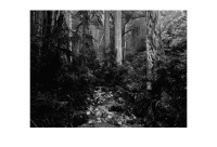
- img = imread ('D: \ Photo \ nature.jpg');
- red = img (:,:, 1);
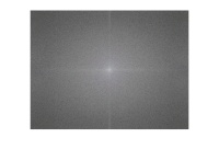
- F = fft2 (img);
- S = fftshift (log (1 + abs (F)));
- S = gscale (S);
- imshow (img), figure, imshow (S);
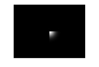
- PQ = paddedsize (size (red));
- [U, V] = dftuv (PQ (1), PQ (2));
- D0 = 0.05 * PQ (2);
- F = fft2 (red, PQ (1), PQ (2));
- H = exp (- (U. ^ 2 + V. ^ 2) / (2 * (D0 ^ 2)));
- g = dftfilt (red, H);
- figure, imshow (fftshift (H), []);
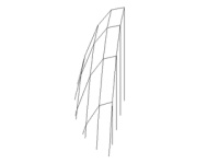
- figure, mesh (H (1: 10: 500, 1: 10: 500))
- axis ([0 50 0 50 0 1])
- colormap (gray)
- grid off
- axis off
- view (-25, 0)
- H = fftshift (hpfilter ('gaussian', 500, 500, 50));
- mesh (H (1: 10: 500, 1: 10: 500))
- axis ([0 50 0 50 0 1])
- colormap ([0 0 0])
- grid off
- axis off
- view (-163, 64)
- figure, imshow (H, []);
- PQ = paddedsize (size (red));
- D0 = 0.05. * PQ (1);
- H = hpfilter ('gaussian', PQ (1), PQ (2), D0);
- g = dftfilt (red, H);
- figure, imshow (g, [0 255]);
- PQ = paddedsize (size (red));
- D0 = 0.05. * PQ (1);
- HBW = hpfilter ('btw', PQ (1), PQ (2), D0.2);
- H = 0.5 + 2 * HBW;
- gbw = dftfilt (red, HBW);
- gbw = gscale (gbw);
- ghf = dftfilt (red, H);
- gbf = gscale (ghf);
- img1 = histeq (red, 256);
- ghe = histeq (ghf, 256);
- figure, imshow (red);
- figure, imshow (ghe, []);
- figure, imshow (img1, []);
**** Examples of work **** Final result


