TAU Darwinism

Foreword

“Cyber ​​Yard Uncle Fedya is exactly three bears in strength,” said Paul, removing the adjustment block from the bowels of the Cyber ​​Yard. “I already know one Fedya here.” Pleasant, freckled. A very, very aseptic young man. Is this not your relative?

Arkady and Boris Strugatsky (Noon. XXII century).

The article is devoted to the applicability of genetic algorithms to the problem of identification of a dynamic system.
Updated: TAU Darwinism Continuation Published : Ruby Implementation

Introduction

The identification of the structure of the mathematical model, as part of the analysis of physical systems, means finding an algebraic expression (equation) that describes the physical model of the object. Many systems identification methods are parametric, i.e. the structure of the model of the identifiable object is determined and, using the given formulas, the parameters of this model are calculated. This article sets out a method for selecting the optimal mathematical model of an object using genetic programming.
The advantage of the GA in this matter is that these algorithms do not limit the list of systems that can be identified with their help and can be applied to any set of data representing the input-output system. When using GA, there is no need to pre-determine the structure of an identifiable object. The optimal structure of the model will be found in the process of evolution of a randomly generated population of individuals (models).

Terminology

• population - a finite set of individuals;
• individual - an organism, a data structure represented by one or more chromosomes, each of which is a point in the multidimensional space of parameters of the problem being solved;
• chromosome - an ordered set of genes;
• gene - characterized by a position in the chromosome and contains the value of some property (parameter);
• genotype - a map of genes for the totality of chromosomes;
• phenotype - a set of possible combinations of genes in a given genotype, i.e. point cloud in the space of task parameters;
• alleles - a set of possible values ​​for each of the genes, i.e. set of values ​​of a specific property;
• locus - the position of the gene in the chromosome.

Identification Object

An inhomogeneous differential equation will be considered as the initial mathematical model of the identifiable object. For simplicity, a second-degree differential equation will be used as an example:

(1)

In the formula (1), “'” (apostrophe) means the time derivative - the operator d / dt; α is the output coordinate (for example, the deviation of the sensing element from the equilibrium position); β - input action, control (for example, the force acting on the SE and leading to its deviation).
In the operator form of writing (s = d / dt), this equation will look like:

(2)

According to expression (2), the transfer function is compiled - the ratio of output to input:

(3)

In (3), the denominator is the “characteristic equation” of the system. It determines the main characteristics of the dynamics (for example, stability). The roots of this equation are called poles of a dynamical system. The roots of the numerator are called the zeros of the dynamical system.
Transfer function (3) can be rewritten in the form of a fraction, the numerator and denominator of which are the products of two and three terms:

(4)

In this case, both the numerator and the denominator each contain one polynomial, but in the general case there will be several of them for equations of order 4 or more. Moreover, each of them corresponds to a point on the complex plane. A point on the real axis corresponds to a binomial, and a point that does not lie on the real axis corresponds to a trinomial. The last statement is true only when the trinomial has only two complex conjugate roots. Otherwise, this trinomial can be represented as the product of two binomials.
In expression (4), the coefficients “T” are time constants, and the coefficient η is the damping decrement (it is also an indicator of the oscillation or damping coefficient).

Genetic coding

To write a mathematical model of an identifiable object in the form (2), it is convenient to use a gene coding scheme with real numbers. In this case, the number of alleles of each gene will be determined by the length (the number of bits of the binary representation) of real numbers in the software implementation of the algorithms.
Let two chromosomes encode a mathematical model of the form (2) - one for the input (right side) and the other for the output (left side). Genes in the chromosomes correspond to one of the terms in equations (2). The value of the gene is equal to the value of the coefficient for variables in the equations. Moreover, the number of genes in the chromosomes can be any. Using this approach, you can encode a system with input and output of any order. As a result, this will allow you to encode a dynamic system with any topology and any number of feedbacks. You only need to follow the rule of physical feasibility - the order of entry is less than or equal to the order of exit.
The disadvantage of this approach is that it is more difficult to control the characteristics of the dynamics. If we compare (3) and (4), it is easy to notice that each of the coefficients in (3) is a combination of several coefficients in (4). Therefore, from the point of view of synthesis of the optimal controller, it may be more advantageous to use the model record in the form (4) even in the context of GA . In this case, the genes will contain the value of the pole or zero PF , and this value will be complex. With this approach to identification using genetic programming, an increase in the resistance of individuals in the population and the rate of convergence of the algorithm to the optimal result is expected.
Regardless of the choice of PF recording formwhen using encoding with real (or complex) numbers, the chromosome will be an array of numbers. You can also introduce binary coding by setting quantization by level and reducing real numbers to integers in the binary representation (“Gray code” [2]). However, often in the transfer functions the adjacent coefficients differ from each other by several orders of magnitude, so problems with accuracy can arise. Another way of binary coding is the logarithmic (also see [2]), in which the first two bits encode the signs of the number and exponent of the power function, and the rest - the value of the exponent itself. Using binary coding, on the one hand, will complicate the algorithm when using complex numbers, but on the other, it will allow the use of classical genetic operators that require binary representation of data.

Fitness function

One of the main concepts in GA is the concept of “fitness function” or “fitness function”. It shows how well the solution presented by this individual satisfies the conditions of the task. In the context of the task of synthesizing the optimal regulator, the quality of regulation can be used as the main criterion for assessing the “fitness” of an individual a good combination of smoothness of the transition process and its duration. In the identification problem, the degree of approximation of the model’s reaction to the input action to the reaction of the real (identifiable) object to the same effect is more important. The degree of approximation can be estimated by the mean-square criterion, calculating the standard deviation of the reaction of the model from the recorded output signal of an identifiable object.

(5)

In expression (5), n is the number of samples in the recorded output signal of an identifiable object; x _cf - the arithmetic mean of the deviation of the reaction of this individual from the output signal of the identified object.
The procedure for calculating the “fitness” of an individual is reduced to the following. First you need to decode the chromosome, i.e. using the values ​​encrypted in it, first create a continuous transfer function (PF with continuous time), and then use this PF to create a discrete model convenient for numerical simulation. It is most convenient for me to use a discrete model in the state space [ 5 ].
At the input of the compiled discrete model, an action is applied that is identical to that applied to the input of the identifiable object. An individual reaction to this effect is recorded. In this case, the model of the individual is compiled with a period of quantization in time equal to the period of quantization of the output signal of the object. Next, you need to use the formula (5), first subtracting the array elements from the resulting array by recording the output signal of the object, after which you can divide the unit by the obtained variance if individuals with higher values ​​of the fitness function are considered more fit.
In addition, a special scaling (for example, power-law) can be introduced into the fitness function so that the most ill-adapted individuals are screened out more slowly. This is necessary to maintain genetic diversity at the proper level. It is also necessary to add an individual viability check. As criteria for such an assessment, the following can be used:

• the order of entry and exit - we do not need models with too much order, as well as models whose order of entry is greater than the order of exit;
• the duration of the transition process - you can approximately estimate the time of PP without conducting a simulation (numerical experiment) with the participation of this model; too long PP also does not suit us;
• overshoot - the ratio of the difference between the maximum reaction and the steady-state value to the steady-state value;
• oscillation - we do not need a model with slowly damping self-oscillations;
• stability - easily determined using the Hurwitz criterion [4].

Crossing and mutation

The publication [2, p. 134] describes a single-point crossing algorithm. It consists in the choice of a locus in which chromosomes “stick together” and the exchange of branches thus obtained between chromosomes occurs. The result is two chromosomes, each of which contains genes from both parents. You can create one individual for each of the chromosomes or only one individual for one of the chromosomes.
The same publication describes a multi-point crossover method. The essence remains the same - sticking points are created and gene chains are recombined. The difference is only in the number of possible combinations of genes and, accordingly, in the number of combined chromosomes obtained. Again, you can create several individuals (optional for each of the chromosomes), but you can only one.
The gene chain exchange algorithm itself can be modified. If instead of simply replacing the values, we use the calculation of some weighted average , then a similarity mechanism of gene competition ( dominant genes and recessive ones ) will be created . The only difference is that the dominance of genes will be determined by the fitness of the individual.
The mutation operator can be implemented by simple calculation of a random value for a randomly selected gene, you can calculate a random increase to the current value of the gene, or you can apply bit inversion. The first method is undesirable, because the values ​​of the coefficients in the transfer functions can vary over a wide range, and a change in the value of one coefficient from very small to large will lead to a sharp change in the value of the fitness function and the loss of stability of the model. A binary mutation has the same danger - a change in the bit responsible for the sign of a number can lead to a loss of stability. Therefore, in this case, the algorithm for calculating a random increase reduced to the current value of the gene is more optimal. This approach means that the range in which a random number is selected is proportional to the current value of the gene. The proportionality coefficient can be selected equal to several units.

Population evolution

On page 211 in [2] a pseudo-code of the evolution of a population is presented:


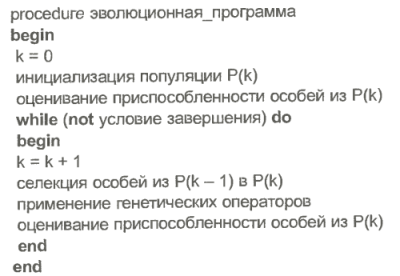
At each iteration step, standard genetic programming procedures are performed on individuals of a population: calculation of fitness functions, selection, crossbreeding, mutation. For the evolution of the population as a whole, the selection process plays a key role. It determines at what speed and whether the population will generally move to a global optimum or become stuck in a local extremum. There are several approaches:

• roulette wheel - each individual is represented on the wheel by a sector whose value is proportional to the value of the fitness function of the individual;
• tournament method - the population is divided into subgroups, within which selection is made according to the value of the fitness function;
• rank method - according to the value of the fitness function of the individual, a rank is assigned, and the higher the rank of the individual, the less its copies will enter the population at the next iteration step;
• combined methods .

It should be noted that it is desirable to introduce a mechanism for protecting individuals with the highest values ​​of the fitness function against accidental elimination. In the classical genetic algorithm, there is little chance that the fittest individual will not enter the new population. Therefore, the individual with the maximum value of the fitness function must be protected from accidental elimination. This strategy is called "elitist".
There is also a strategy for transferring some individuals to a new population without applying genetic operations to them, i.e. parents do not die immediately after the birth of the offspring. In addition to this strategy, you can introduce an age penalty into the fitness function, i.e. a decrease in its value is proportional to the age of the individual.
Another important modification of GA is “niche”. In accordance with it, a coefficient is added to the fitness function that is inversely proportional to the number and proximity of neighbors in the multidimensional space of optimized parameters. As a result, the modified fitness function will look like:

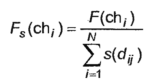(6)

If an individual is in its niche alone, i.e. If there are no neighbors similar to it, then the value of the fitness function will not be changed. Otherwise, its value will be reduced in proportion to the proximity and the number of neighbors in the niche. Moreover, the degree of proximity can be estimated in various ways.
The introduction of niche allows us to find several extrema, i.e. several optimal models at once, close in dynamics characteristics to an identifiable object, but at the same time differing from each other.

Conclusion

In conclusion, I would like to say that at present, genetic algorithms, along with various modifications, some of which are considered in this article, and evolutionary strategies are combined under one common name “evolutionary algorithms”. Initially, genetic algorithms and evolutionary strategies developed independently of each other. But later, experts began to combine techniques from these two areas. Currently, the difference between them is not so noticeable. Much of what was stated in the article would be more correct to attribute to evolutionary strategies, but for simplicity of perception, it was decided to leave everything as it is.

Thanks for attention! Your comments ...

Update 1: at the request of readers, I am expanding the list of references.

List of references

1. Stephan WINKLER, Michael AFFENZELLER, Stefan WAGNER . NEW METHODS FOR THE IDENTIFICATION OF NONLINEAR MODEL STRUCTURES BASED UPON GENETIC PROGRAMMING TECHNIQUES // Institute of Systems Theory and Simulation, Johannes Kepler University Linz, Austria {winkler, ma, sw} @ cast.uni-linz.ac.at
2. Rutkovskaya D ., Pilinsky M., Rutkovsky L. Neural networks, genetic algorithms and fuzzy systems: Per. from polish I. D. Rudinsky. - M .: Hot line - Telecom, 2006. - 452 p.: Ill.
3. The Voronoi move
4. Routh-Hurwitz stability criterion
5. State space (control theory)
6. Concepts of the practical use of genetic algorithms
7."Hello world!" using genetic algorithms
8. Genetic algorithm
9. Evolutionary algorithms