October 7, 2010 at 10:55
Data compression in industrial automation systems. SwingingDoor Algorithm
Hello dear readers. I want to bring to your attention a description of the SwingingDoor data compression algorithm and talk about how we use it.
By occupation, I am engaged in the development of solutions in the field of industrial automation, and more specifically - in the development of production information systems. Their purpose is to provide information for people and other systems. They provide up-to-date, up-to-date data as well as historical data. Data comes from numerous control systems (SC), the number of parameters is measured in tens of thousands.
Why use compression, why not store all the data?
The reasons are fairly obvious:
Of course, hard drives with a large amount of memory are now available and communication channels are getting better and better, but, let's be realistic, these issues cannot be ignored. In addition, as will be said below, storing the entire amount of data does not always make sense.
By the way, sparse data can be used instead of compression (the average value of the parameter for the period), but these values will already differ from the "raw" data obtained from control systems. The averaged data will smooth out the instantaneous maximum and minimum parameter values. For some tasks, this is acceptable, but for part it is not.
One of the tasks of our system is the consolidation of data from various company ICs into a single database.
Some SCs, such as telemechanics, provide data every second, while the data itself may not change significantly.
For example, if you look at the graph below, we will see that the values of the “Total generation by CHP” parameter vary from 11.5 to 12.5 MW, while in most cases the neighboring values differ from each other by less than 0.1, and the general dynamics of changes has some regularity.
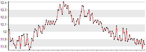
In order not to store "extra" data, we can skip part of the samples. Compression consists precisely in the selection of “necessary” data from the input stream.
General compression requirements:
• thinned data should not change the general idea of the process;
• all local extrema of the graph must with certain accuracy be present in the thinned data — in other words, if a sharp jump in the parameter value occurs, the algorithm should fix this.
These criteria can be formulated more strictly. For example (and this criterion will be used in the following algorithm), the decimation method should ensure that if we save two points and skip several points between them, then the line connecting the saved points will be separated from these points by no more than a given error.
The green line graph below shows the points that will remain after applying compression.
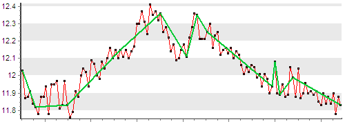
There is also another requirement for compression algorithms. Since they process a large amount of data, they should work quickly. Ideally (and this is implemented in the following algorithm), they should work with the data stream and, without returning to the previously obtained points, make a decision on archiving the last considered point.
For data compression, we use the SwingingDoor algorithm. The algorithm was patented in the USA in May 1987. The main field of application of the algorithm is process control systems and production information systems.
The algorithm is called the “Revolving Door”. The name of the algorithm reflects the principle of operation.
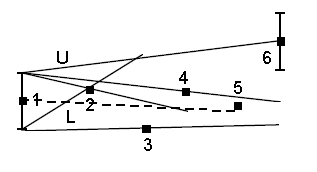
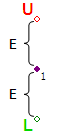
Step # 1 - Get the first point. At a distance of equal error E, we postpone vertically two reference points L and U.
Step # 2 - Get the second point. Through the reference points L, U and the resulting point, we draw rays. The rays form the doors of the corridor.

Step # 3 - Point 3 does not enter the corridor constructed in the second step. We rotate the ray L clockwise to point 3.

Step # 4 - Point 4 does not enter the corridor constructed in the previous step. Rotate the U ray counterclockwise to point 4

Step # 5 - Point 5 enters the corridor, do nothing
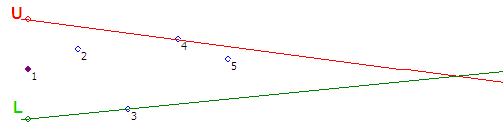
Step # 6 - Point 6 does not enter the corridor. We begin to rotate the beam U counterclockwise until it intersects point 6 and we find that the doors of the corridor opened

Step # 7 - Open a new corridor, starting from point 5. Save points 1 and 5.

Out of the first 5 points, only two will be saved. In Example 3, the points were “redundant” for us, which allowed us to cut off 60% of the input data.
In the specification of the algorithm, it is proposed to start a new corridor from a point located between points 5 and 6 and distant from the beam U at E / 2. But in our project, we proceed differently - we begin to build a new corridor from the last point that enters the corridor, i.e. from point 5, because with this behavior we guarantee that all thinned data will have a time stamp and value obtained from the control system.
Using data compression allowed us to:
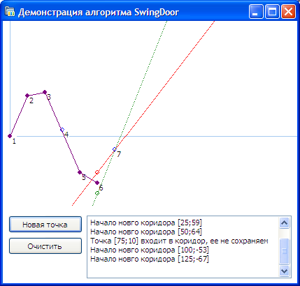
Before implementing the algorithm, we wrote an application simulating the operation of the algorithm. Here you can download the source code (Delphi) of the demo application.
US-Patent-4669097 - Data compression for display and storage
By occupation, I am engaged in the development of solutions in the field of industrial automation, and more specifically - in the development of production information systems. Their purpose is to provide information for people and other systems. They provide up-to-date, up-to-date data as well as historical data. Data comes from numerous control systems (SC), the number of parameters is measured in tens of thousands.
Why use compression, why not store all the data?
Data compression
The reasons are fairly obvious:
- to reduce disk space for data storage;
- to reduce the load of data channels.
Of course, hard drives with a large amount of memory are now available and communication channels are getting better and better, but, let's be realistic, these issues cannot be ignored. In addition, as will be said below, storing the entire amount of data does not always make sense.
By the way, sparse data can be used instead of compression (the average value of the parameter for the period), but these values will already differ from the "raw" data obtained from control systems. The averaged data will smooth out the instantaneous maximum and minimum parameter values. For some tasks, this is acceptable, but for part it is not.
How do we use data compression
One of the tasks of our system is the consolidation of data from various company ICs into a single database.
Some SCs, such as telemechanics, provide data every second, while the data itself may not change significantly.
For example, if you look at the graph below, we will see that the values of the “Total generation by CHP” parameter vary from 11.5 to 12.5 MW, while in most cases the neighboring values differ from each other by less than 0.1, and the general dynamics of changes has some regularity.
In order not to store "extra" data, we can skip part of the samples. Compression consists precisely in the selection of “necessary” data from the input stream.
General compression requirements:
• thinned data should not change the general idea of the process;
• all local extrema of the graph must with certain accuracy be present in the thinned data — in other words, if a sharp jump in the parameter value occurs, the algorithm should fix this.
These criteria can be formulated more strictly. For example (and this criterion will be used in the following algorithm), the decimation method should ensure that if we save two points and skip several points between them, then the line connecting the saved points will be separated from these points by no more than a given error.
The green line graph below shows the points that will remain after applying compression.
There is also another requirement for compression algorithms. Since they process a large amount of data, they should work quickly. Ideally (and this is implemented in the following algorithm), they should work with the data stream and, without returning to the previously obtained points, make a decision on archiving the last considered point.
SwingingDoor Algorithm
For data compression, we use the SwingingDoor algorithm. The algorithm was patented in the USA in May 1987. The main field of application of the algorithm is process control systems and production information systems.
Principle of operation
The algorithm is called the “Revolving Door”. The name of the algorithm reflects the principle of operation.
Step # 1 - Get the first point. At a distance of equal error E, we postpone vertically two reference points L and U.
Step # 2 - Get the second point. Through the reference points L, U and the resulting point, we draw rays. The rays form the doors of the corridor.
Step # 3 - Point 3 does not enter the corridor constructed in the second step. We rotate the ray L clockwise to point 3.
Step # 4 - Point 4 does not enter the corridor constructed in the previous step. Rotate the U ray counterclockwise to point 4
Step # 5 - Point 5 enters the corridor, do nothing
Step # 6 - Point 6 does not enter the corridor. We begin to rotate the beam U counterclockwise until it intersects point 6 and we find that the doors of the corridor opened
Step # 7 - Open a new corridor, starting from point 5. Save points 1 and 5.
Out of the first 5 points, only two will be saved. In Example 3, the points were “redundant” for us, which allowed us to cut off 60% of the input data.
In the specification of the algorithm, it is proposed to start a new corridor from a point located between points 5 and 6 and distant from the beam U at E / 2. But in our project, we proceed differently - we begin to build a new corridor from the last point that enters the corridor, i.e. from point 5, because with this behavior we guarantee that all thinned data will have a time stamp and value obtained from the control system.
Algorithm Setting
- Error E - sets the maximum possible deviation of the corridor points from the resulting line (along the Y axis). In the picture above, this line is between points 1 and 5. The error must be set for each parameter separately, based on its meaning. For example, generation surges from 10 to 10.2 MW are acceptable, but a frequency jump from 50 to 50.2 Hz is a serious violation. Therefore, for generation, the error can be set, for example, equal to 0.1, and for the frequency - 0.01.
- Corridor lifetime is the time during which at least one point must be saved. Variants of the process are possible when the data may not change significantly (air temperature on a frosty winter night). In this case, they will fall into the current corridor of permissible values and the algorithm will not make a decision on their preservation. To avoid such cases, an appropriate parameter is introduced, which is responsible for how long the data within one corridor can not be stored. For example, for data with a refresh rate of 1 second, you can specify this parameter equal to 30 seconds, thereby providing at least one value in the thinned graph for 30 seconds.
Conclusion
Using data compression allowed us to:
- provide employees of the enterprise with "raw" trends of parameters that were obtained from the UK months ago;
- reduce disk storage space;
- reduce the load of data transmission channels;
- optimize data collection services from the enterprise IC, thereby reducing the load on the CPU of servers on which data collection services are installed.
Demo application
Before implementing the algorithm, we wrote an application simulating the operation of the algorithm. Here you can download the source code (Delphi) of the demo application.
Materials
US-Patent-4669097 - Data compression for display and storage