The use of neural networks in image recognition
Quite a lot has already been said about neural networks, as one of the tools for solving difficultly formalized tasks. And here, on the hub, it was shown how to use these networks for image recognition, in relation to the task of breaking captcha. However, there are quite a few types of neural networks. And is a classic fully connected neural network (PNS) so good for the task of recognizing (classifying) images?
So, we are going to solve the problem of image recognition. This can be recognition of faces, objects, characters, etc. To begin with, I propose to consider the problem of recognizing handwritten numbers. This task is good for a number of reasons:
It is proposed to use the MNIST database as input . This database contains 60,000 training pairs (image - label) and 10,000 test pairs (images without labels). Images are normalized in size and centered. The size of each figure is no more than 20x20, but they are inscribed in a square 28x28 in size. An example of the first 12 digits from the training set of the MNIST database is shown in the figure:

Thus, the task is formulated as follows: create and train a neural network for handwriting recognition, taking their images at the input and activating one of 10 outputs . By activation, we mean the value 1 at the output. The values of the remaining outputs in this case should (ideally) be equal to -1. Why this scale is not used [0,1] I will explain later.
Most people refer to “ordinary” or “classic” neural networks as direct-

coupled fully connected neural networks with backward propagation of error: As the name implies in each network, each neuron is connected to each, the signal goes only in the direction from the input layer to the output, there are no recursions. We will call such a network in abbreviated form PNS.
First you need to decide how to submit data to the input. The simplest and almost non-alternative solution for PNS is to express a two-dimensional image matrix in the form of a one-dimensional vector. Those. for the image of a handwritten figure 28x28 in size, we will have 784 inputs, which is not enough. What happens next is why many conservative scientists do not like neural networks and their methods - the choice of architecture. And they don’t like it, because the choice of architecture is pure shamanism. There are still no methods to uniquely determine the structure and composition of the neural network based on the description of the problem. In defense, I’ll say that for hardly formalized tasks it is unlikely that such a method will ever be created. In addition, there are many different network reduction techniques (for example, OBD [1]), as well as various heuristics and rules of thumb. One such rule states that the number of neurons in the hidden layer should be at least an order of magnitude greater than the number of inputs. If we take into account that the conversion from an image to an indicator of a class is rather complicated and essentially non-linear, it is not enough to do one layer here. Based on the foregoing, we roughly estimate that the number of neurons in the hidden layers will be of the order of15,000 (10,000 in the 2nd layer and 5,000 in the third). At the same time, for a configuration with two hidden layers, the number of configurable and trained links will be 10 million between the inputs and the first hidden layer + 50 million between the first and second + 50 thousand between the second and output, if we assume that we have 10 outputs, each of which denotes a number from 0 to 9. Total roughly 60 million connections . I have not in vain mentioned that they are customizable - this means that during training for each of them it will be necessary to calculate the error gradient.
Well, okay, what can you do,beautyartificial intelligence requires sacrifice. But if you think about it, it comes to mind that when we convert the image into a linear chain of bytes, we will irretrievably lose something. Moreover, with each layer, this loss is only exacerbated. So it is - we are losing the topology of the image, i.e. the relationship between its individual parts. In addition, the task of recognition implies the ability of the neural network to be resistant to small shifts, rotations and zooming, i.e. it must extract certain invariants from the data that are not dependent on the handwriting of a particular person. So what should be a neural network to be not very computationally complex and, at the same time, more invariant to various image distortions?
The solution to this problem was found by French-born American scientist Jan LeCun , inspired by the work of Nobel laureates in the field of medicine Torsten Nils Wiesel and David H. Hubel . These scientists examined the visual cortex of a cat’s brain and found that there are so-called simple cells that respond especially strongly to straight lines at different angles and complex cells that respond to lines moving in one direction. Ian LeKun suggested using the so-called convolutional neural networks [2].
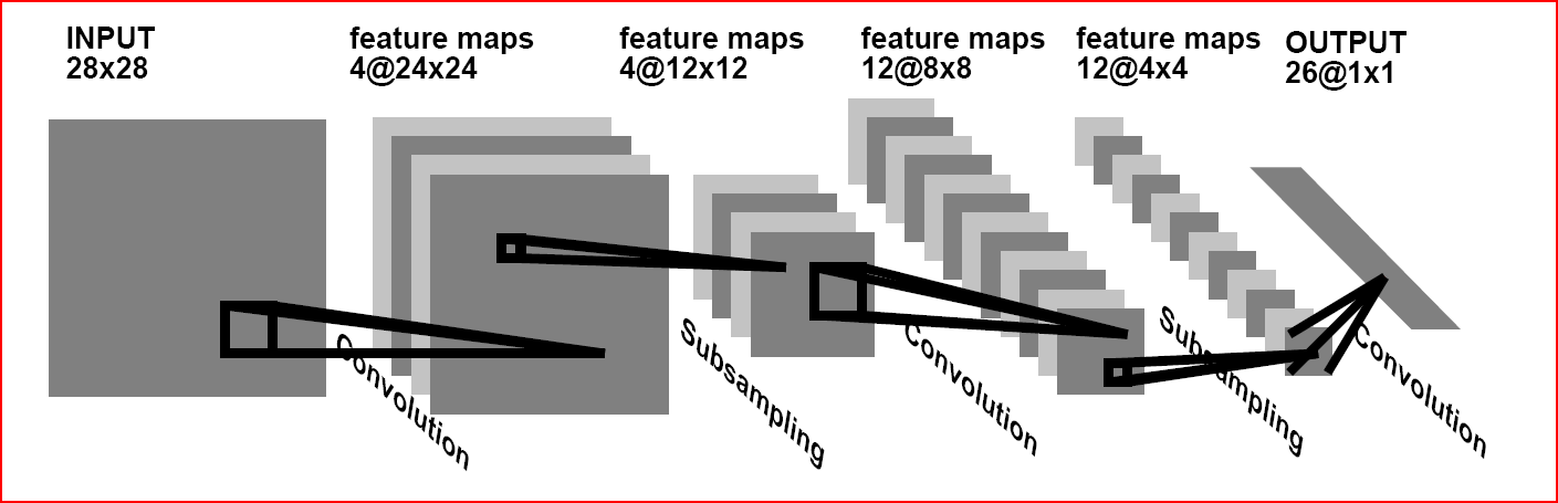
The idea of convolutional neural networks is to alternate convolutional layers (C-layers), subsampling layers (S-layers) and the presence of fully connected (F-layers) layers at the output.
This architecture contains 3 main paradigms:
Local perception implies that at the input of one neuron, not the whole image (or the outputs of the previous layer) is supplied, but only some of its area. This approach allowed us to preserve the topology of the image from layer to layer.
The concept of shared weights suggests that a very small set of weights is used for a large number of ties. Those. if we have an input image of 32x32 pixels in size, then each of the neurons in the next layer will accept only a small section of this image, for example, 5x5, with each of the fragments being processed with the same set. It is important to understand that there can be many sets of scales themselves, but each of them will be applied to everythingimage. Such sets are often called kernels. It is easy to calculate that even for 10 cores of size 5x5 for an input image of size 32x32 the number of links will be approximately 256,000 (compare with 10 million), and the number of tunable parameters is only 250!
But what, you ask, will this affect the quality of recognition? Oddly enough, for the better. The fact is that such an artificial weight restriction improves the generalization properties of the network (generalization), which ultimately positively affects the ability of the network to find invariants in the image and react mainly to them, not paying attention to other noise. You can look at this approach from a slightly different perspective. Those who studied the classics of image recognition and know how it works in practice (for example, in military equipment) know that most of these systems are based on two-dimensional filters. A filter is a matrix of coefficients, usually specified manually. This matrix is applied to the image using a mathematical operation called convolution.. The essence of this operation is that each image fragment is multiplied by the matrix (core) of convolution element by element and the result is summed and written to the same position in the output image. The main property of such filters is that the value of their output is greater the more the image fragment resembles the filter itself. Thus, the image convoluted with a certain core will give us another image, each pixel of which will indicate the degree of similarity of the image fragment to the filter. In other words, it will be a feature map.
The process of signal propagation in the C-layer, I tried to depict in the figure:
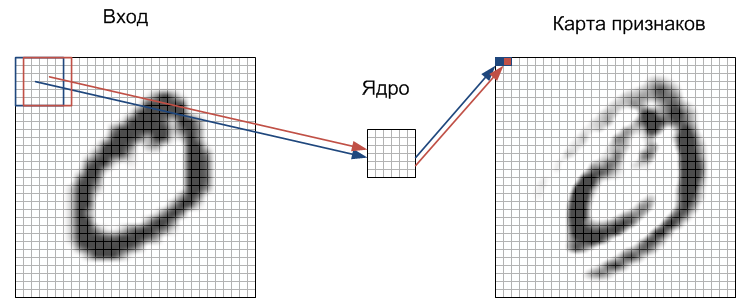
Each image fragment is element-wise multiplied by a small matrix of weights (core), the result is summed. This amount is a pixel of the output image, which is called a feature map. Here I omitted the fact that the weighted sum of inputs is still passed through the activation function (as in any other neural network). In fact, this can happen in the S-layer, there is no fundamental difference. It should be said that, ideally, not different fragments pass sequentially through the core, but in parallel the entire image passes through identical nuclei. In addition, the number of cores (sets of weights) is determined by the developer and depends on how many features must be selected. Another feature of the convolutional layer is that it slightly reduces the image due to edge effects.
The essence of downsamplingand S-layers is to reduce the spatial dimension of the image. Those. the input image is roughly (averaged) reduced by a specified number of times. Most often 2 times, although there may be an uneven change, for example, 2 vertically and 3 horizontally. Sub-sampling is needed to ensure scale invariance.
Alternating layers allows you to create feature maps from feature maps, which in practice means the ability to recognize complex feature hierarchies.
Usually, after passing through several layers, a feature map degenerates into a vector or even a scalar, but there are hundreds of feature maps. In this form, they are fed to one or two layers of a fully connected network. The output layer of such a network may have various activation functions. In the simplest case, it can be a tangential function; radial basis functions are also successfully used.
In order to start training our network, you need to decide how to measure the quality of recognition. In our case, for this we will use the most common mean square error (MSE) function in neural network theory [3]:
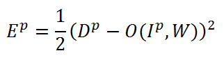
In this formula, Ep is the recognition error for the pth training pair, Dp is the desired network output, O (Ip, W) - network output, depending on the p-th input and weight coefficients W, which includes convolution kernels, displacements, weight coefficients of S- and F-layers. The task of training is to adjust the weights W so that for any training pair (Ip, Dp) they give a minimum error Ep. To calculate the error for the entire training sample, we simply take the arithmetic mean of the errors for all training pairs. We denote this average error as E.
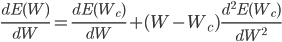
To minimize the error function Ep, the most effective are gradient methods. Consider the essence of gradient methods using the simplest one-dimensional case as an example (i.e. when we have only one weight). If we expand the error function Ep in the Taylor series, we get the following expression:

Here E is the same error function, Wc is some initial weight value. From school mathematics, we remember that in order to find the extremum of a function, it is necessary to take its derivative and equate to zero. So let's do it, take the derivative of the error function by weight, discarding the terms above the second order:
from this expression it follows that the weight at which the value of the error function will be minimal can be calculated from the following expression:
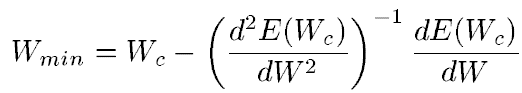
Those. the optimal weight is calculated as the current minus the derivative of the error function by weight divided by the second derivative of the error function. For the multidimensional case (i.e., for the weight matrix), everything is exactly the same, only the first derivative turns into a gradient (vector of partial derivatives), and the second derivative turns into Hessian (matrix of second partial derivatives). And here two options are possible. If we omit the second derivative, we get the algorithm of the fastest gradient descent. If we still want to take into account the second derivative, then we’ll be stunned by how much computing resources we need to calculate the full Hessian, and then reverse it. Therefore, usually Hessian is replaced by something simpler. For example, one of the most famous and successful methods - the Levenberg-Marquardt (LM) method replaces the Hessian,Details here I will not tell.
But what is important for us to know about these two methods is that the LM algorithm requires the processing of the entire training sample, while the gradient descent algorithm can work with each individual training sample. In the latter case, the algorithm is called a stochastic gradient. Given that our database contains 60,000 training samples, a stochastic gradient is more suitable for us. Another advantage of the stochastic gradient is its lower susceptibility to falling into a local minimum compared to LM.
There is also a stochastic modification of the LM algorithm, which I may mention later.
The formulas presented make it easy to calculate the derivative of the error with respect to the weights in the output layer. The error propagation method, widely known in AI, allows calculating errors in hidden layers .
Personally, I use Matlab to implement various algorithms that are not required to operate in real time. This is a very convenient package, the M-language of which allows you to focus on the algorithm itself without worrying about memory allocation, I / O operations, etc. In addition, many different toolboxes allow you to create truly interdisciplinary applications in the shortest possible time. You can, for example, use the Image Acquisition Toolbox to connect a webcam, use the Image Processing Toolbox to process an image from it, use the Neural Network Toolbox to form the robot's motion path, and use the Virtual Reality Toolbox and Control Systems Toolbox to simulate the robot’s movement. Speaking of the Neural Network Toolbox, this is a fairly flexible set of tools that allows you to create many neural networks of various types and architectures, but, unfortunately, not convolutional NS. It's all about shared scales. NN toolbox does not have the ability to set shared weights.
To eliminate this drawback, I wrote a class that allows you to implement the SNA of arbitrary architecture and apply them to various tasks. Download the class here . The class itself was written so that to the one who uses it the maximum network structure is visible. Everything is very plentifully commented on, on the name of variables did not save. The network simulation speed is not bad and is a fraction of a second. The speed of training is not yet large (> 10 hours), but stay tuned, acceleration by orders is planned in the near future.
Those who are interested in implementing the SNA in C ++ can find it here and here .
The program on matlabcentral comes with a file of an already trained neural network, as well as a GUI for demonstrating the results of work. The following are examples of recognition:

The link contains a table comparing recognition methods based on MNIST. The first place is for convolutional neural networks with the result of 0.39% recognition errors [4]. Most of these mistakenly recognized images are not recognized by every person correctly. In addition, elastic distortions of input images, as well as preliminary training without a teacher, were used in [4]. But about these methods in some other article.
PS Thank you all for your comments and feedback. This is my first article on the hub, so I will be glad to see suggestions, comments, additions.
1. The challenge
So, we are going to solve the problem of image recognition. This can be recognition of faces, objects, characters, etc. To begin with, I propose to consider the problem of recognizing handwritten numbers. This task is good for a number of reasons:
- To recognize a handwritten symbol, it is quite difficult to compile a formalized (not intellectual) algorithm, and this becomes clear, you just have to look at the same number written by different people
- The task is quite relevant and is related to OCR (optical character recognition)
- There is a freely available base of handwritten characters available for download and experimentation.
- There are quite a few articles on this subject and it is very easy and convenient to compare different approaches.
It is proposed to use the MNIST database as input . This database contains 60,000 training pairs (image - label) and 10,000 test pairs (images without labels). Images are normalized in size and centered. The size of each figure is no more than 20x20, but they are inscribed in a square 28x28 in size. An example of the first 12 digits from the training set of the MNIST database is shown in the figure:
Thus, the task is formulated as follows: create and train a neural network for handwriting recognition, taking their images at the input and activating one of 10 outputs . By activation, we mean the value 1 at the output. The values of the remaining outputs in this case should (ideally) be equal to -1. Why this scale is not used [0,1] I will explain later.
2. "Normal" neural networks.
Most people refer to “ordinary” or “classic” neural networks as direct-
coupled fully connected neural networks with backward propagation of error: As the name implies in each network, each neuron is connected to each, the signal goes only in the direction from the input layer to the output, there are no recursions. We will call such a network in abbreviated form PNS.
First you need to decide how to submit data to the input. The simplest and almost non-alternative solution for PNS is to express a two-dimensional image matrix in the form of a one-dimensional vector. Those. for the image of a handwritten figure 28x28 in size, we will have 784 inputs, which is not enough. What happens next is why many conservative scientists do not like neural networks and their methods - the choice of architecture. And they don’t like it, because the choice of architecture is pure shamanism. There are still no methods to uniquely determine the structure and composition of the neural network based on the description of the problem. In defense, I’ll say that for hardly formalized tasks it is unlikely that such a method will ever be created. In addition, there are many different network reduction techniques (for example, OBD [1]), as well as various heuristics and rules of thumb. One such rule states that the number of neurons in the hidden layer should be at least an order of magnitude greater than the number of inputs. If we take into account that the conversion from an image to an indicator of a class is rather complicated and essentially non-linear, it is not enough to do one layer here. Based on the foregoing, we roughly estimate that the number of neurons in the hidden layers will be of the order of15,000 (10,000 in the 2nd layer and 5,000 in the third). At the same time, for a configuration with two hidden layers, the number of configurable and trained links will be 10 million between the inputs and the first hidden layer + 50 million between the first and second + 50 thousand between the second and output, if we assume that we have 10 outputs, each of which denotes a number from 0 to 9. Total roughly 60 million connections . I have not in vain mentioned that they are customizable - this means that during training for each of them it will be necessary to calculate the error gradient.
Well, okay, what can you do,
3. Convolutional neural networks
The solution to this problem was found by French-born American scientist Jan LeCun , inspired by the work of Nobel laureates in the field of medicine Torsten Nils Wiesel and David H. Hubel . These scientists examined the visual cortex of a cat’s brain and found that there are so-called simple cells that respond especially strongly to straight lines at different angles and complex cells that respond to lines moving in one direction. Ian LeKun suggested using the so-called convolutional neural networks [2].
The idea of convolutional neural networks is to alternate convolutional layers (C-layers), subsampling layers (S-layers) and the presence of fully connected (F-layers) layers at the output.
This architecture contains 3 main paradigms:
- Local perception.
- Shared Weights.
- Downsampling.
Local perception implies that at the input of one neuron, not the whole image (or the outputs of the previous layer) is supplied, but only some of its area. This approach allowed us to preserve the topology of the image from layer to layer.
The concept of shared weights suggests that a very small set of weights is used for a large number of ties. Those. if we have an input image of 32x32 pixels in size, then each of the neurons in the next layer will accept only a small section of this image, for example, 5x5, with each of the fragments being processed with the same set. It is important to understand that there can be many sets of scales themselves, but each of them will be applied to everythingimage. Such sets are often called kernels. It is easy to calculate that even for 10 cores of size 5x5 for an input image of size 32x32 the number of links will be approximately 256,000 (compare with 10 million), and the number of tunable parameters is only 250!
But what, you ask, will this affect the quality of recognition? Oddly enough, for the better. The fact is that such an artificial weight restriction improves the generalization properties of the network (generalization), which ultimately positively affects the ability of the network to find invariants in the image and react mainly to them, not paying attention to other noise. You can look at this approach from a slightly different perspective. Those who studied the classics of image recognition and know how it works in practice (for example, in military equipment) know that most of these systems are based on two-dimensional filters. A filter is a matrix of coefficients, usually specified manually. This matrix is applied to the image using a mathematical operation called convolution.. The essence of this operation is that each image fragment is multiplied by the matrix (core) of convolution element by element and the result is summed and written to the same position in the output image. The main property of such filters is that the value of their output is greater the more the image fragment resembles the filter itself. Thus, the image convoluted with a certain core will give us another image, each pixel of which will indicate the degree of similarity of the image fragment to the filter. In other words, it will be a feature map.
The process of signal propagation in the C-layer, I tried to depict in the figure:
Each image fragment is element-wise multiplied by a small matrix of weights (core), the result is summed. This amount is a pixel of the output image, which is called a feature map. Here I omitted the fact that the weighted sum of inputs is still passed through the activation function (as in any other neural network). In fact, this can happen in the S-layer, there is no fundamental difference. It should be said that, ideally, not different fragments pass sequentially through the core, but in parallel the entire image passes through identical nuclei. In addition, the number of cores (sets of weights) is determined by the developer and depends on how many features must be selected. Another feature of the convolutional layer is that it slightly reduces the image due to edge effects.
The essence of downsamplingand S-layers is to reduce the spatial dimension of the image. Those. the input image is roughly (averaged) reduced by a specified number of times. Most often 2 times, although there may be an uneven change, for example, 2 vertically and 3 horizontally. Sub-sampling is needed to ensure scale invariance.
Alternating layers allows you to create feature maps from feature maps, which in practice means the ability to recognize complex feature hierarchies.
Usually, after passing through several layers, a feature map degenerates into a vector or even a scalar, but there are hundreds of feature maps. In this form, they are fed to one or two layers of a fully connected network. The output layer of such a network may have various activation functions. In the simplest case, it can be a tangential function; radial basis functions are also successfully used.
4. Training
In order to start training our network, you need to decide how to measure the quality of recognition. In our case, for this we will use the most common mean square error (MSE) function in neural network theory [3]:
In this formula, Ep is the recognition error for the pth training pair, Dp is the desired network output, O (Ip, W) - network output, depending on the p-th input and weight coefficients W, which includes convolution kernels, displacements, weight coefficients of S- and F-layers. The task of training is to adjust the weights W so that for any training pair (Ip, Dp) they give a minimum error Ep. To calculate the error for the entire training sample, we simply take the arithmetic mean of the errors for all training pairs. We denote this average error as E.
To minimize the error function Ep, the most effective are gradient methods. Consider the essence of gradient methods using the simplest one-dimensional case as an example (i.e. when we have only one weight). If we expand the error function Ep in the Taylor series, we get the following expression:
Here E is the same error function, Wc is some initial weight value. From school mathematics, we remember that in order to find the extremum of a function, it is necessary to take its derivative and equate to zero. So let's do it, take the derivative of the error function by weight, discarding the terms above the second order:
from this expression it follows that the weight at which the value of the error function will be minimal can be calculated from the following expression:
Those. the optimal weight is calculated as the current minus the derivative of the error function by weight divided by the second derivative of the error function. For the multidimensional case (i.e., for the weight matrix), everything is exactly the same, only the first derivative turns into a gradient (vector of partial derivatives), and the second derivative turns into Hessian (matrix of second partial derivatives). And here two options are possible. If we omit the second derivative, we get the algorithm of the fastest gradient descent. If we still want to take into account the second derivative, then we’ll be stunned by how much computing resources we need to calculate the full Hessian, and then reverse it. Therefore, usually Hessian is replaced by something simpler. For example, one of the most famous and successful methods - the Levenberg-Marquardt (LM) method replaces the Hessian,Details here I will not tell.
But what is important for us to know about these two methods is that the LM algorithm requires the processing of the entire training sample, while the gradient descent algorithm can work with each individual training sample. In the latter case, the algorithm is called a stochastic gradient. Given that our database contains 60,000 training samples, a stochastic gradient is more suitable for us. Another advantage of the stochastic gradient is its lower susceptibility to falling into a local minimum compared to LM.
There is also a stochastic modification of the LM algorithm, which I may mention later.
The formulas presented make it easy to calculate the derivative of the error with respect to the weights in the output layer. The error propagation method, widely known in AI, allows calculating errors in hidden layers .
5. Implementation
Personally, I use Matlab to implement various algorithms that are not required to operate in real time. This is a very convenient package, the M-language of which allows you to focus on the algorithm itself without worrying about memory allocation, I / O operations, etc. In addition, many different toolboxes allow you to create truly interdisciplinary applications in the shortest possible time. You can, for example, use the Image Acquisition Toolbox to connect a webcam, use the Image Processing Toolbox to process an image from it, use the Neural Network Toolbox to form the robot's motion path, and use the Virtual Reality Toolbox and Control Systems Toolbox to simulate the robot’s movement. Speaking of the Neural Network Toolbox, this is a fairly flexible set of tools that allows you to create many neural networks of various types and architectures, but, unfortunately, not convolutional NS. It's all about shared scales. NN toolbox does not have the ability to set shared weights.
To eliminate this drawback, I wrote a class that allows you to implement the SNA of arbitrary architecture and apply them to various tasks. Download the class here . The class itself was written so that to the one who uses it the maximum network structure is visible. Everything is very plentifully commented on, on the name of variables did not save. The network simulation speed is not bad and is a fraction of a second. The speed of training is not yet large (> 10 hours), but stay tuned, acceleration by orders is planned in the near future.
Those who are interested in implementing the SNA in C ++ can find it here and here .
6. Results
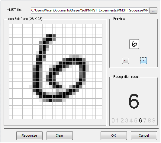
The program on matlabcentral comes with a file of an already trained neural network, as well as a GUI for demonstrating the results of work. The following are examples of recognition:
The link contains a table comparing recognition methods based on MNIST. The first place is for convolutional neural networks with the result of 0.39% recognition errors [4]. Most of these mistakenly recognized images are not recognized by every person correctly. In addition, elastic distortions of input images, as well as preliminary training without a teacher, were used in [4]. But about these methods in some other article.
References
- Yann LeCun, JS Denker, S. Solla, RE Howard and LD Jackel: Optimal Brain Damage, in Touretzky, David (Eds), Advances in Neural Information Processing Systems 2 (NIPS * 89), Morgan Kaufman, Denver, CO, 1990
- Y. LeCun and Y. Bengio: Convolutional Networks for Images, Speech, and Time-Series, in Arbib, MA (Eds), The Handbook of Brain Theory and Neural Networks, MIT Press, 1995
- Y. LeCun, L. Bottou, G. Orr and K. Muller: Efficient BackProp, in Orr, G. and Muller K. (Eds), Neural Networks: Tricks of the trade, Springer, 1998
- Ranzato Marc'Aurelio, Christopher Poultney, Sumit Chopra and Yann LeCun: Efficient Learning of Sparse Representations with an Energy-Based Model, in J. Platt et al. (Eds), Advances in Neural Information Processing Systems (NIPS 2006), MIT Press, 2006
PS Thank you all for your comments and feedback. This is my first article on the hub, so I will be glad to see suggestions, comments, additions.