July 22, 2019 at 08:56
Uniform distribution of points on a sphere
- Transfer
The most uniform distribution of points on the sphere is an incredibly important task in mathematics, science, and computer systems, and applying a Fibonacci grid to the surface of the sphere using the same projection is an extremely fast and efficient approximation method for solving it. I will show how, with minor changes, it can be made even better.
Some time ago this post appeared on the Hacker News homepage. Its discussion can be read here .
The problem of uniform distribution of points on a sphere has a very long history. This is one of the most well-studied problems in the mathematical literature on spherical geometry. It is of critical importance in many areas of mathematics, physics, chemistry, including computational methods, approximation theory, coding theory, crystallography, electrostatics, computer graphics, virus morphology and many others.
Unfortunately, with the exception of a few special cases (namely, Platonic solids), it is impossible to perfectly distribute points on a sphere. In addition, the solution of the problem strongly depends on the criterion that is used to assess uniformity. In practice, many criteria are used , including:
It is very important to clarify this aspect: usually there is no single optimal solution to this problem, because an optimal solution based on one criterion is often not an optimal distribution of points for others. For example, we will also find out that packaging optimization does not necessarily create an optimal convex hull and vice versa.
For the sake of brevity, in this post we will consider only two criteria: the minimum packing distance and the convex hull / Delaunay mesh (volume and area).
In section 1, we show how you can change the canonical Fibonacci grid to build an improved distribution of packaging . In Section 2, we show how you can change the canonical Fibonacci grid to build improved parameters for convex hulls. (volume and surface area).
Often this problem is called the Tamm's task in honor of the botanist Tems, who sought an explanation of the surface structure of pollen grains. The packing criterion requires us to maximize the smallest distance between neighbors for points. I.e
This value decreases with speed. , therefore, it will be useful to determine the normalized distance, as well as the asymptotic limit of the normalized distance, as
Fibonacci grid
One very elegant solution models the nodes found in nature, for example, the distribution of seeds in a sunflower or pine cone. This phenomenon is called spiral phyllotaxis . Coxeter showed that such structures have a fundamental connection with the Fibonacci series, and the golden ratio
  .
.
In the literature, two similar definitions of the set of points of a spherical Fibonacci grid are found. The source is defined strictly forequal to one of the members of the Fibonacci series,  , and well studied in number theory.
The second definition generalizes the formula to an arbitrary amount and is used in calculations more often:
Where
Below is an example of the same Fibonacci grids. By transformation, you can turn these sets of points into Fibonacci spirals that are well known to us.
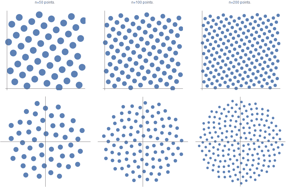
Similarly, these sets of points can be transferred from the unit square![$ [0, 1] ^ 2 $](https://habrastorage.org/getpro/habr/formulas/446/120/9fb/4461209fb31a93beb7f34775d0b85091.svg) on a sphere using a cylindrical isometric projection:
on a sphere using a cylindrical isometric projection:
Many different versions of Python code for it can be found on stackoverflow: Evenly distributing points on a sphere .
Even despite the fact that spherical Fibonacci sets are globally not the best distribution of samples on a sphere (because their solutions do not coincide with the solutions for Platonic solids for ), they have excellent sampling properties and are very easy to build compared to other, more complex spherical sampling schemes.
Since the transfer from the unit square to the surface of the sphere is carried out by a projection with conservation of area, it can be expected that if the starting points are distributed evenly, they will also be fairly well distributed on the surface of the sphere. However, this does not mean that the distribution will be provably optimal.
This transfer suffers from two different but interrelated problems.
Firstly, this overlay is performed while maintaining the area, not the distance. Given that in our case, the condition is to maximize the minimum pairwise distance between points, such conditions and relationships will not necessarily be satisfied after projection.
The second problem is most difficult to solve from a practical point of view: the superposition has two degenerate points at each pole. Consider two points that are very close to the pole, but differing by 180 degrees in longitude. On a single square (and on a cylindrical projection) they will correspond to two points very distant from each other, but when superimposed on the surface of a sphere they can be connected by a very small arc passing through the north pole. Because of this particular problem, many spiral overlays are not optimal enough.
The Fibonacci Spherical Helix obtained from Equation 1 gives the value for all , i.e
  .
.
Grid 1
A more common version (especially on computer systems) that creates a better value has the form:
It places the points at the midpoints of the intervals (according to the midpoint rule in the Gauss quadratic formula), therefore, for , the values of the first coordinate will be as follows:
Grid 2.
The key to further improving Equation 2 is the realization that always corresponds to the distance between points  and
and  that are at the poles. That is, to improve
 points near the poles should be spaced even further.
If we define the following distribution:
- curves for various values.  (blue);
  (orange);
  (green); and
 (red). You can see thatgives results closer to asymptotic results. That is, with
 The following simple expression generates significantly better results.
  compared to the canonical spherical Fibonacci grid:
That is, with the values of the first coordinate will be equal to:
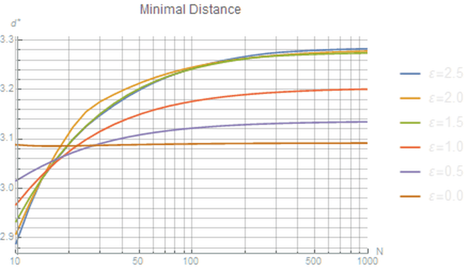
Figure 1. Different values at different values  . The higher the value, the more optimal the configuration. We see that
 provides a solution close to optimal.
Grid 3.
As mentioned above, one of the most serious problems of uniform distribution of points on a sphere is that the distribution optimality critically depends on the objective function used. It turns out. that local quantities likesometimes they almost “do not forgive mistakes” - a single point in an insufficiently optimal position can catastrophically reduce the assessment of the entire distribution of points.
In our case, regardless of the magnitude value  usually defined by the four points closest to each of the poles, especially and . However, it is also known about this grid that the largest Voronoi polygon is at the pole. So trying to maximizeby dividing the original polar points in a row, we actually increase the void at the pole even more! Therefore, we presented an alternative to grid 2, which is generally preferable because it does not show such a large void near the poles.
It is almost identical to grid 2, but has two differences. First, she uses at
at  . Secondly, besides these
 The first and last points are located at each of the poles.
I.e:
An amazing property of this construction method is that despite the fact that its creation was motivated by a desire to minimize voids at the poles, it actually has the best value among all methods and  from
from  !
!
That is, with the values of the first coordinate will be as follows:
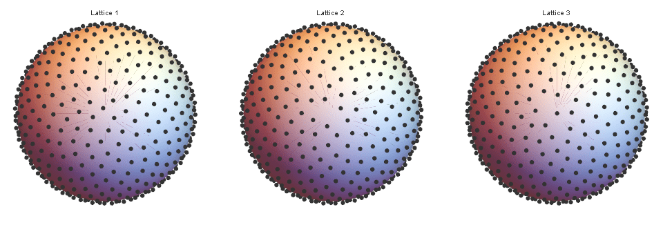
Figure 2. Various grid configurations. The canonical Fibonacci grid on the left. Note that even though the middle gridimproved, at the pole she has a noticeable void. Grid 3 has no void at the pole and has the best value.
Comparison
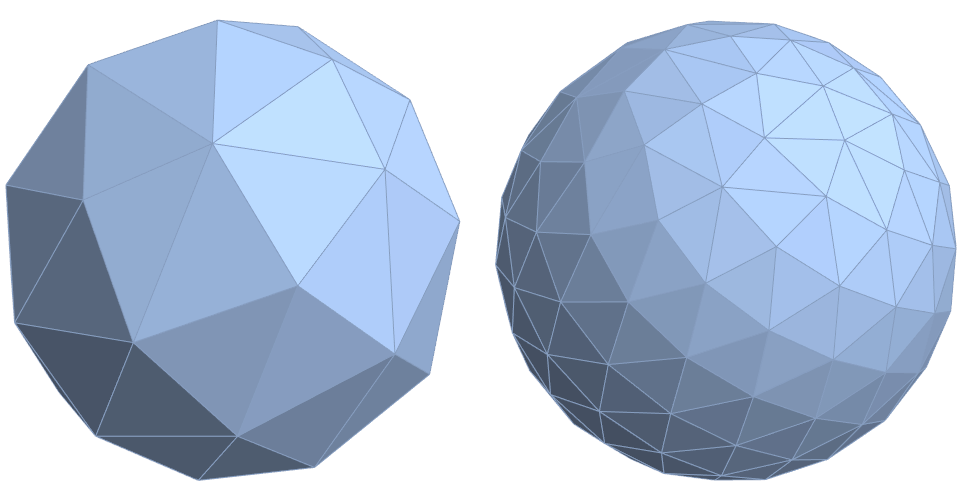
At large values this value extremely well comparable with other methods, for example, geodesic domes, which are based on triangulated projections from the faces of Platonic solids onto the surface of a sphere. It is not surprising that the highest quality geodesic domes are built on the basis of the icosahedron or dodecahedron.
Icosahedron-based geodesic domes at various values.
Dodecahedron-based geodesic domes for various values.
In addition, a truncated icosahedron corresponding to the shape of fullerene has only
  .
.
That is, with mesh based on equation 3 is better than any geodesic polyhedron.
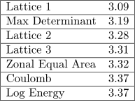
According to the data from the first source in the list of references below, some of the modern methods, which are usually complex and require recursive and / or dynamic programming, have the following indicators.
Conclusion from Section 1
In the previous section, we optimized the distribution byHowever, these modifications worsen other indicators, for example, the volume of a convex hull (Delaunay mesh). This section describes how to evenly distribute points on a sphere in such a way as to optimize (maximize) such a more global indicator as the volume of a convex hull.
We denote like a convex hull points
normalization factor included, because the absolute discrepancy decreases with speed  .
.
Behavior at various can be seen in Figure 3 (blue line).
To reduce the mismatch of volumes, it should be noted that despite the use of , from the logic of the golden section at
  it does not necessarily follow that it is the best value for the final . Speaking scientifically, we can say that we need to take into account the influence of limb limb correction.
Let's summarize equation 1 as follows:
where we define as
as
Where
Where - the function of rounding to the nearest integer down.
Figure 3 shows how much volume mismatch is optimized for half of the values..
The reason for this is a little-known fact: all numbers satisfying the special Mobius transformation, starting from irrationality, are equivalent .
Therefore, the reason that and  fit together so well, is that
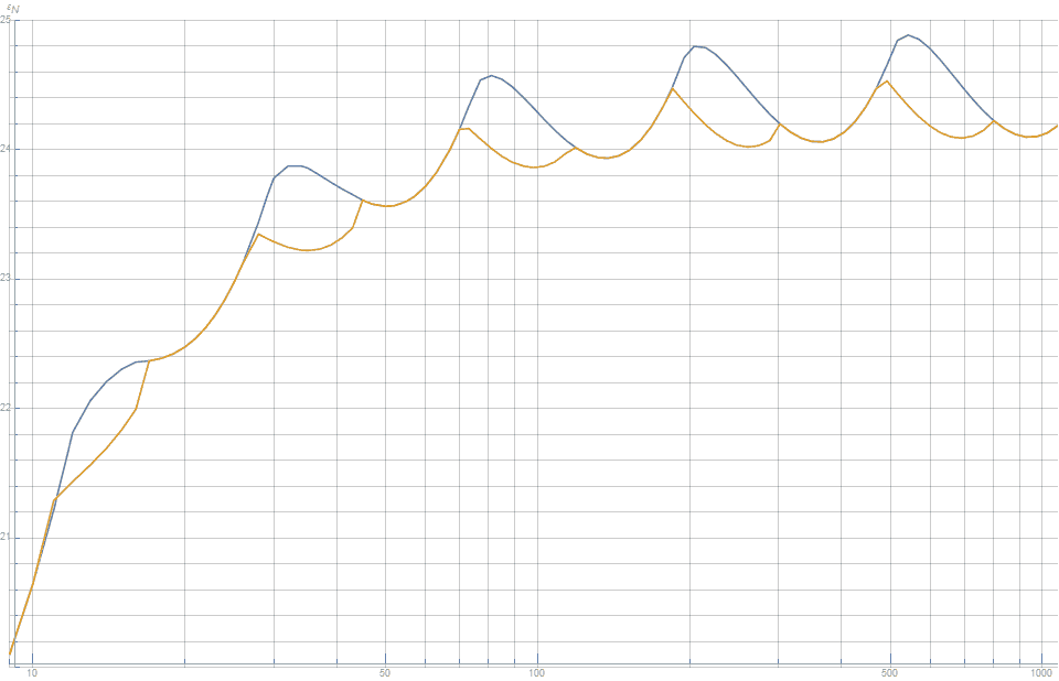
Figure 3. The mismatch between the volume of the convex hull of points and the volume of the unit sphere. Keep in mind that the smaller it is, the better. The figure shows that the hybrid model (orange line) based on and , provides a better distribution of points than the canonical Fibonacci grid (blue line).
For the remaining half, we first define an auxiliary series being a variation of the Fibonacci series
I.e
All fractions of this series have elegant continuous fractions, and in the limit converge to. For instance,
Now we can fully generalize in the following way:
The table below shows the values for various .
Figure 4 shows that with respect to the volume of the convex hull, this new distribution is better than the canonical grid for all values
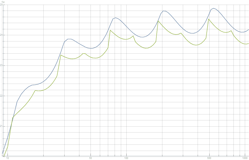
Figure 4. The mismatch between the volume of the convex hull and the volume of the unit sphere. The lower the value, the better. This tells us that the proposed new method (green line) constantly provides a better distribution than the canonical Fibonacci grid (blue line).
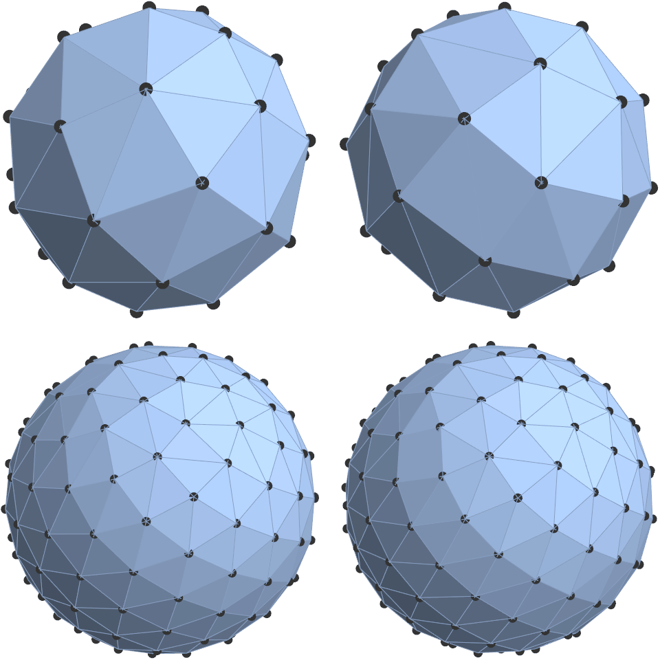
Figure 5. Visual comparison of the canonical mesh (left) with the new modified mesh (right) with n = 35 and n = 150. Visually, the differences are almost imperceptible. However, in conditions requiring maximum efficiency, the modified version (on the right) provides a small, but quantifiable improvement in both volume and surface area of the convex hull.
Curiously, this distribution is also insignificant, but steadily reduces the mismatch between the surface area of the convex hull and the surface area of a single sphere. This is shown in Figure 6.
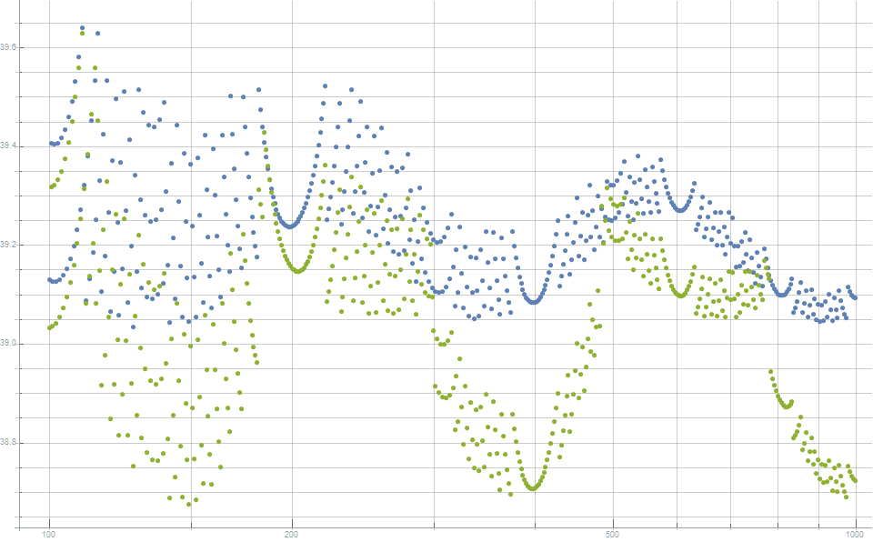
Рисунок 5. Нормализованное рассогласование площадей между площадью поверхности выпуклой оболочки (сетки Делоне) и площадью поверхности единичной сферы. Чем ниже значения, тем лучше. Это показывает, что предложенная новая модификация (зелёные точки) демонстрирует небольшое, но постоянное снижение разности площадей поверхностей по сравнению с канонической сеткой Фибоначчи (синие точки)
Вывод из раздела 2
Источники
Some time ago this post appeared on the Hacker News homepage. Its discussion can be read here .
Introduction
The problem of uniform distribution of points on a sphere has a very long history. This is one of the most well-studied problems in the mathematical literature on spherical geometry. It is of critical importance in many areas of mathematics, physics, chemistry, including computational methods, approximation theory, coding theory, crystallography, electrostatics, computer graphics, virus morphology and many others.
Unfortunately, with the exception of a few special cases (namely, Platonic solids), it is impossible to perfectly distribute points on a sphere. In addition, the solution of the problem strongly depends on the criterion that is used to assess uniformity. In practice, many criteria are used , including:
- Packaging and coating
- Convex hulls, Voronoi cells and Delaunay triangles
- Kernels
 Rice Energy
 - Cubature and qualifiers
It is very important to clarify this aspect: usually there is no single optimal solution to this problem, because an optimal solution based on one criterion is often not an optimal distribution of points for others. For example, we will also find out that packaging optimization does not necessarily create an optimal convex hull and vice versa.
For the sake of brevity, in this post we will consider only two criteria: the minimum packing distance and the convex hull / Delaunay mesh (volume and area).
In section 1, we show how you can change the canonical Fibonacci grid to build an improved distribution of packaging . In Section 2, we show how you can change the canonical Fibonacci grid to build improved parameters for convex hulls. (volume and surface area).
Section 1. Optimization of packaging distance
Often this problem is called the Tamm's task in honor of the botanist Tems, who sought an explanation of the surface structure of pollen grains. The packing criterion requires us to maximize the smallest distance between neighbors for
points. I.e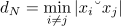
This value decreases with speed.
, therefore, it will be useful to determine the normalized distance, as well as the asymptotic limit of the normalized distance, as
Fibonacci grid
One very elegant solution models the nodes found in nature, for example, the distribution of seeds in a sunflower or pine cone. This phenomenon is called spiral phyllotaxis . Coxeter showed that such structures have a fundamental connection with the Fibonacci series,
and the golden ratio . In the literature, two similar definitions of the set of points of a spherical Fibonacci grid are found. The source is defined strictly for
equal to one of the members of the Fibonacci series, , and well studied in number theory.
The second definition generalizes the formula to an arbitrary amount
and is used in calculations more often:
Where
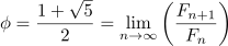
Below is an example of the same Fibonacci grids. By transformation, you can turn these sets of points into Fibonacci spirals that are well known to us.

Similarly, these sets of points can be transferred from the unit square
on a sphere using a cylindrical isometric projection:

Many different versions of Python code for it can be found on stackoverflow: Evenly distributing points on a sphere .
Even despite the fact that spherical Fibonacci sets are globally not the best distribution of samples on a sphere (because their solutions do not coincide with the solutions for Platonic solids for
), they have excellent sampling properties and are very easy to build compared to other, more complex spherical sampling schemes. Since the transfer from the unit square to the surface of the sphere is carried out by a projection with conservation of area, it can be expected that if the starting points are distributed evenly, they will also be fairly well distributed on the surface of the sphere. However, this does not mean that the distribution will be provably optimal.
This transfer suffers from two different but interrelated problems.
Firstly, this overlay is performed while maintaining the area, not the distance. Given that in our case, the condition is to maximize the minimum pairwise distance between points, such conditions and relationships will not necessarily be satisfied after projection.
The second problem is most difficult to solve from a practical point of view: the superposition has two degenerate points at each pole. Consider two points that are very close to the pole, but differing by 180 degrees in longitude. On a single square (and on a cylindrical projection) they will correspond to two points very distant from each other, but when superimposed on the surface of a sphere they can be connected by a very small arc passing through the north pole. Because of this particular problem, many spiral overlays are not optimal enough.
The Fibonacci Spherical Helix obtained from Equation 1 gives the value
for all , i.e . Grid 1
A more common version (especially on computer systems) that creates a better value
has the form:
It places the points at the midpoints of the intervals (according to the midpoint rule in the Gauss quadratic formula), therefore, for
, the values of the first coordinate will be as follows:
Grid 2.
The key to further improving Equation 2 is the realization that
always corresponds to the distance between points and that are at the poles. That is, to improvepoints near the poles should be spaced even further. If we define the following distribution:

- curves for various values. (blue); (orange); (green); and(red). You can see thatgives results closer to asymptotic results. That is, with The following simple expression generates significantly better results. compared to the canonical spherical Fibonacci grid:
That is, with
the values of the first coordinate will be equal to:
Figure 1. Different values
at different values . The higher the value, the more optimal the configuration. We see thatprovides a solution close to optimal. Grid 3.
As mentioned above, one of the most serious problems of uniform distribution of points on a sphere is that the distribution optimality critically depends on the objective function used. It turns out. that local quantities like
sometimes they almost “do not forgive mistakes” - a single point in an insufficiently optimal position can catastrophically reduce the assessment of the entire distribution of points. In our case, regardless of the magnitude
value usually defined by the four points closest to each of the poles, especially and . However, it is also known about this grid that the largest Voronoi polygon is at the pole. So trying to maximizeby dividing the original polar points in a row, we actually increase the void at the pole even more! Therefore, we presented an alternative to grid 2, which is generally preferable because it does not show such a large void near the poles. It is almost identical to grid 2, but has two differences. First, she uses
at . Secondly, besides theseThe first and last points are located at each of the poles. I.e:

An amazing property of this construction method is that despite the fact that its creation was motivated by a desire to minimize voids at the poles, it actually has the best value among all methods
and from ! That is, with
the values of the first coordinate will be as follows:
Figure 2. Various grid configurations. The canonical Fibonacci grid on the left. Note that even though the middle grid
improved, at the pole she has a noticeable void. Grid 3 has no void at the pole and has the best value. Comparison
At large values
this value extremely well comparable with other methods, for example, geodesic domes, which are based on triangulated projections from the faces of Platonic solids onto the surface of a sphere. It is not surprising that the highest quality geodesic domes are built on the basis of the icosahedron or dodecahedron. Icosahedron-based geodesic domes at various values
.
Dodecahedron-based geodesic domes for various values
.
In addition, a truncated icosahedron corresponding to the shape of fullerene
has only . That is, with
mesh based on equation 3 is better than any geodesic polyhedron. According to the data from the first source in the list of references below, some of the modern methods, which are usually complex and require recursive and / or dynamic programming, have the following indicators.
Conclusion from Section 1
Grid 3, created by Equation 3, is a modification of the canonical Fibonacci grid, which provides much better packaging for the distribution of points. I.e

Section 2. Optimization of the convex hull (Delaunay mesh)
In the previous section, we optimized the distribution by
However, these modifications worsen other indicators, for example, the volume of a convex hull (Delaunay mesh). This section describes how to evenly distribute points on a sphere in such a way as to optimize (maximize) such a more global indicator as the volume of a convex hull. We denote
like a convex hull points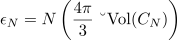
normalization factor included
, because the absolute discrepancy decreases with speed . Behavior
at various can be seen in Figure 3 (blue line). To reduce the mismatch of volumes, it should be noted that despite the use of
, from the logic of the golden section at it does not necessarily follow that it is the best value for the final . Speaking scientifically, we can say that we need to take into account the influence of limb limb correction. Let's summarize equation 1 as follows:

where we define
as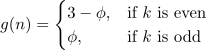
Where

Where
- the function of rounding to the nearest integer down. Figure 3 shows how much volume mismatch is optimized for half of the values.
. The reason for this is a little-known fact: all numbers
satisfying the special Mobius transformation, starting from irrationality, are equivalent .
Therefore, the reason that
and fit together so well, is that
Figure 3. The mismatch between the volume of the convex hull of points and the volume of the unit sphere. Keep in mind that the smaller it is, the better. The figure shows that the hybrid model (orange line) based on
and , provides a better distribution of points than the canonical Fibonacci grid (blue line). For the remaining half, we first define an auxiliary series
being a variation of the Fibonacci series
I.e

All fractions of this series have elegant continuous fractions, and in the limit converge to
. For instance,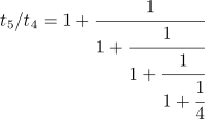
Now we can fully generalize
in the following way:
The table below shows the values
for various .
Figure 4 shows that with respect to the volume of the convex hull, this new distribution is better than the canonical grid for all values
Figure 4. The mismatch between the volume of the convex hull and the volume of the unit sphere. The lower the value, the better. This tells us that the proposed new method (green line) constantly provides a better distribution than the canonical Fibonacci grid (blue line).
Figure 5. Visual comparison of the canonical mesh (left) with the new modified mesh (right) with n = 35 and n = 150. Visually, the differences are almost imperceptible. However, in conditions requiring maximum efficiency, the modified version (on the right) provides a small, but quantifiable improvement in both volume and surface area of the convex hull.
Curiously, this distribution is also insignificant, but steadily reduces the mismatch between the surface area of the convex hull and the surface area of a single sphere. This is shown in Figure 6.
Рисунок 5. Нормализованное рассогласование площадей между площадью поверхности выпуклой оболочки (сетки Делоне) и площадью поверхности единичной сферы. Чем ниже значения, тем лучше. Это показывает, что предложенная новая модификация (зелёные точки) демонстрирует небольшое, но постоянное снижение разности площадей поверхностей по сравнению с канонической сеткой Фибоначчи (синие точки)
Вывод из раздела 2
Сетка, соответствующая уравнению 6, является модификацией канонической сетки Фибоначчи, создающей значительно лучшее распределение точек, исходя из объёма и площади поверхности выпуклой оболочки (сетки Делоне).
Источники
- A Comparison of popular point confugrations on S^2“:
- web.archive.org/web/20120421191837
- www.cgafaq.info/wiki/Evenly_distributed_points_on_sphere
- perswww.kuleuven.be/~u0017946/publications/Papers97/art97a-Saff-Kuijlaars-MI/Saff-Kuijlaars-MathIntel97.pdf
- projecteuclid.org/download/pdf_1/euclid.em/1067634731
- maths-people.anu.edu.au/~leopardi/Leopardi-Sphere-PhD-Thesis.pdf
- www.irit.fr/~David.Vanderhaeghe/M2IGAI-CO/2016-g1/docs/spherical_fibonacci_mapping.pdf
- arxiv.org/pdf/1407.8282.pdf
- maths-people.anu.edu.au/~leopardi/Macquarie-sphere-talk.pdf