July 18, 2019 at 08:15
Lecture course "Fundamentals of Digital Signal Processing"
Hello!
Often people turn to me with questions on tasks from the field of digital signal processing (DSP). I tell in detail the nuances, suggest the necessary sources of information. But all listeners, as time has shown, lack practical tasks and examples in the process of learning this area. In this regard, I decided to write a short interactive course on digital signal processing and put it in the public domain .
Most of the training material for visual and interactive presentation is implemented using the Jupyter Notebook . It is assumed that the reader has basic knowledge of the field of higher mathematics, as well as a little command of the Python programming language.

This course contains materials in the form of finished lectures on various topics from the field of digital signal processing. Materials are presented using Python libraries (numpy, scipy, matplotlib packages, etc.). The basic information for this course was taken from my lectures, which I, as a graduate student, gave to students of the Moscow Energy Institute (NRU MEI). Part of the information from these lectures was used at training seminars at the Center for Contemporary Electronics , where I acted as a lecturer. In addition, this material includes the translation of various scientific articles, compilation of information from reliable sources and literature on digital signal processing, as well as official documentation on application packages and built-in functions of the scipy and numpy libraries of Python.
For MATLAB (GNU Octave) users, mastering the material from the point of view of program code is not difficult, since the main functions and their attributes are largely identical and similar to the methods from the Python libraries.
All materials are grouped by the main topics of digital signal processing:
The list of lectures is sufficientbut, of course, incomplete for an introductory acquaintance with the field of DSP. With free time, I plan to support and develop this project.
All materials are absolutely free and available as an open repository on my github as an opensource project . Materials are presented in two formats - in the form of Jupyter Notebooks for interactive work, study and editing, and in the form of HTML files compiled from these notebooks (after downloading from the github they have a quite suitable format for reading and printing).
The following is a very brief description of the sections of the course with short explanations, terms and definitions. Basic information is available in the initial lectures, here is only a brief overview!
Introductory section, which contains basic information on the types of signals. The concept of a discrete sequence, delta function and Heaviside function (unit jump) is introduced.
All signals according to the method of presentation on the set can be divided into four groups:
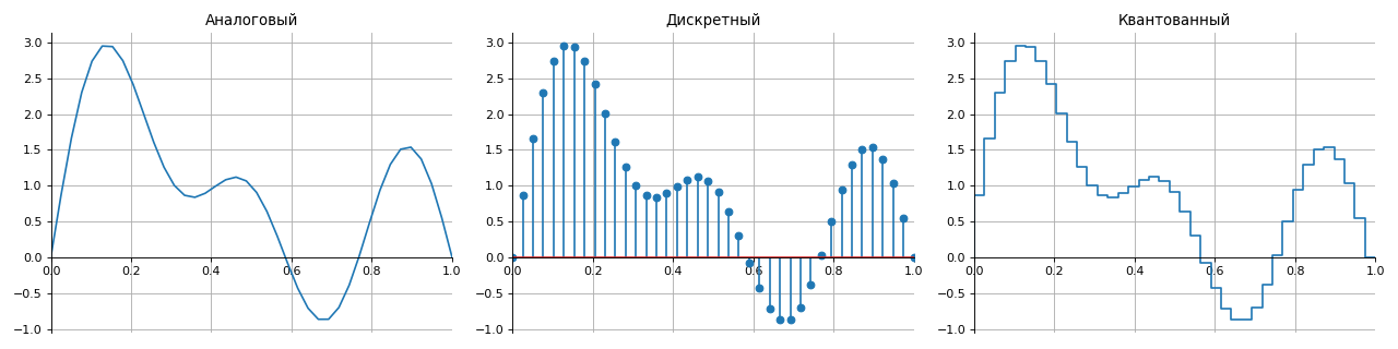
For the correct reconstruction of an analog signal from a digital one without distortion and loss, the sampling theorem known as the Kotelnikov (Nyquist-Shannon) theorem is used .
Such an interpretation is valid provided that the continuous function of time occupies a frequency band from 0 to the value of the upper frequency. If the quantization and discretization steps are chosen incorrectly, the signal will be distorted from analog to discrete.
Also in this section, the Z-transformation and its properties are described, and the representation of discrete sequences in the Z-form is shown.
Example of a finite discrete sequence:
An example of the same sequence in the Z-form:
X (z) = 2 + z -1 - 2z -2 + 2z -4 + 3z -5 + 1z -6
This section describes the concept of the time and frequency domain of a signal. The definition of the discrete Fourier transform (DFT) is introduced. The direct and inverse DFTs and their main properties are considered. Shown is the transition from the DFT to the fast Fourier transform (FFT) algorithm in base 2 (decimation algorithms in frequency and time). Reflected the effectiveness of FFT in comparison with DFT.
In particular, this section describes the Python package scipy.ffpack for computing various Fourier transforms (sine, cosine, direct, inverse, multidimensional, real).
The Fourier transform allows you to represent any function as a set of harmonic signals! The Fourier transform is the basis of convolution methods and the design of digital correlators, is actively used in spectral analysis, and is used when working with long numbers.
Features of the spectra of discrete signals:
1. The spectral density of a discrete signal is a periodic function with a period equal to the sampling frequency.
2. If the discrete sequence is real , then the spectral density modulus of such a sequence is an even function, and the argument is an odd frequency function.
Harmonic Signal Spectrum:
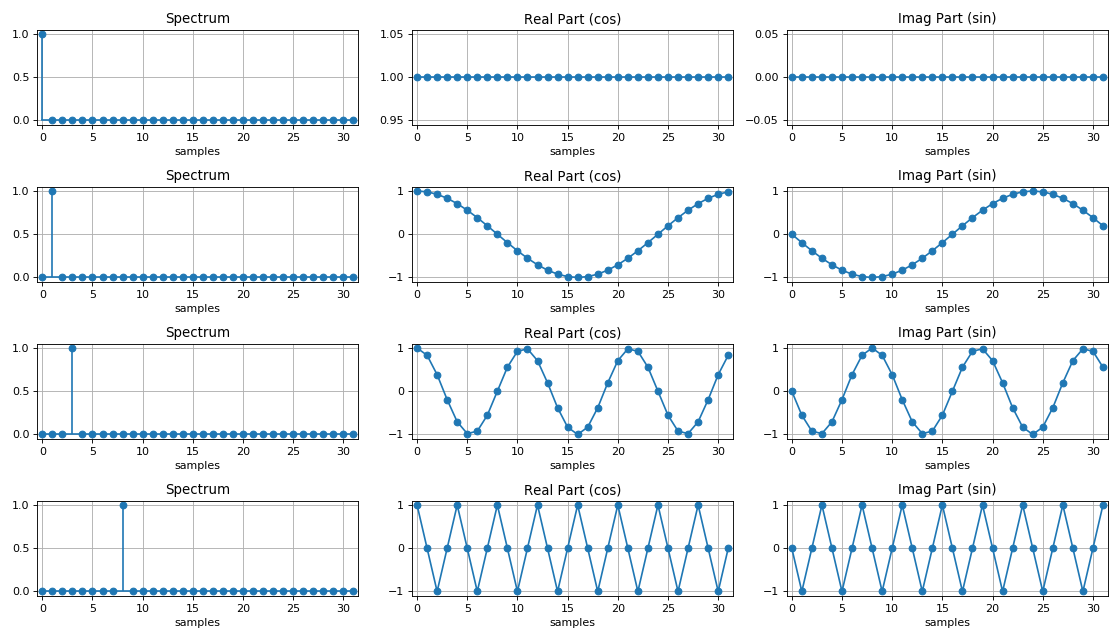
The efficiency of the FFT algorithm and the number of operations performed linearly depends on the sequence length N:
As you can see, the longer the conversion length, the greater the savings in computing resources (in terms of processing speed or the number of hardware units)!
Any arbitrary waveform can be represented as a set of harmonic signals of different frequencies. In other words, a signal of complex shape in the time domain has a set of complex samples in the frequency domain, which are called * harmonics *. These samples express the amplitude and phase of the harmonic effect at a specific frequency. The larger the set of harmonics in the frequency domain, the more accurately the complex waveform appears.

This section introduces the concept of correlation and convolution for discrete random and deterministic sequences. The relationship between autocorrelation and cross-correlation functions with convolution is shown. The properties of convolution are described, in particular, the methods of linear and cyclic convolution of a discrete signal with detailed analysis on the example of a discrete sequence are considered. In addition, a method for computing “fast” convolution using FFT algorithms is shown.
In real problems, the question is often raised about the degree of similarity of one process to another or about the independence of one process from another. In other words, it is necessary to determine the relationship between the signals, that is, to find the correlation. Correlation methods are used in a wide range of tasks: signal search, computer vision and image processing, in radar problems to determine the characteristics of targets and determine the distance to an object. In addition, correlation is used to search for weak signals in noise.
The convolution describes the interaction of signals with each other. If one of the signals is the impulse response of the filter, then the convolution of the input sequence with the impulse response is nothing but a reaction of the circuit to the input action. In other words, the resulting signal reflects the passage of the signal through the filter.
Autocorrelation function(ACF) is used in coding information. The choice of the coding sequence according to the parameters of length, frequency and shape is largely due to the correlation properties of this sequence. The best code sequence has the lowest probability of false detection or operation (for detecting signals, for threshold devices) or false synchronization (for transmitting and receiving code sequences).
This section presents a table comparing the effectiveness of fast convolution and convolution calculated by the direct formula (by the number of real multiplications).
As you can see, for FFT lengths up to 64, fast convolution loseshave a direct method. However, with an increase in the FFT length, the results change in the opposite direction - a quick convolution begins to outperform the direct method. Obviously, the longer the FFT, the better the gain in the frequency method.
In this section, the concept of random signals, probability density, random distribution law is introduced. Mathematical moments are considered - mean (mathematical expectation) and variance (or the root of this quantity is the standard deviation). Also in this section, the normal distribution and the related concept of white noise are considered as the main source of noise (interference) during signal processing.
A random signal is a function of time whose values are not known in advance and can only be predicted with some probability . The main characteristics of random signals include:
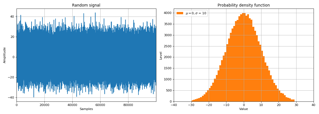
In DSP tasks, random signals are divided into two classes:
Using random variables, we can simulate the effect of a real medium on the passage of a signal from a source to a data receiver. When a signal passes through some noisy link, the so-called white noise is added to the signal. As a rule, the spectral density of such noise is uniformly (equally) distributed at all frequencies, and the noise values in the time domain are normally distributed (Gaussian distribution law). Since white noise is physically added to the signal amplitudes in the selected time samples, it is called Additive white Gaussian noise (AWGN).
This section shows the basic methods for changing one or more parameters of a harmonic signal. The concepts of amplitude, frequency and phase modulation are introduced. In particular, the linear frequency modulation used in radar problems is highlighted. The main characteristics of the signals, the spectra of the modulated signals depending on the modulation parameters are shown.

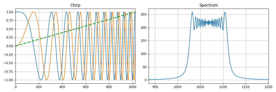
For convenience, a set of functions has been created in Python that implements the above types of modulation. Example of chirp signal implementation:
Also in this section from the theory of transmission of discrete messages types of digital modulation - manipulations are described. As in the case of analog signals, digital harmonic sequences can be manipulated in amplitude, phase and frequency (or several parameters at once).

A sufficiently large section devoted to digital filtering of discrete sequences. In digital signal processing tasks, data flows through circuits called filters . Digital filters, like analog ones, have different characteristics - frequency: frequency response, phase response, time: impulse response, as well as the transfer characteristic of the filter. Digital filters are mainly used to improve signal quality — to isolate a signal from a data sequence, or to degrade unwanted signals — to suppress certain signals in incoming sample sequences.

The section lists the main advantages and disadvantages of digital filters (compared to analog). The concept of impulse and transfer characteristics of the filter is introduced. Two classes of filters are considered - with an infinite impulse response (IIR) and a finite impulse response (FIR). A method for designing filters in canonical and direct form is shown . For FIR filters, the question of how to switch to a recursive form is considered.
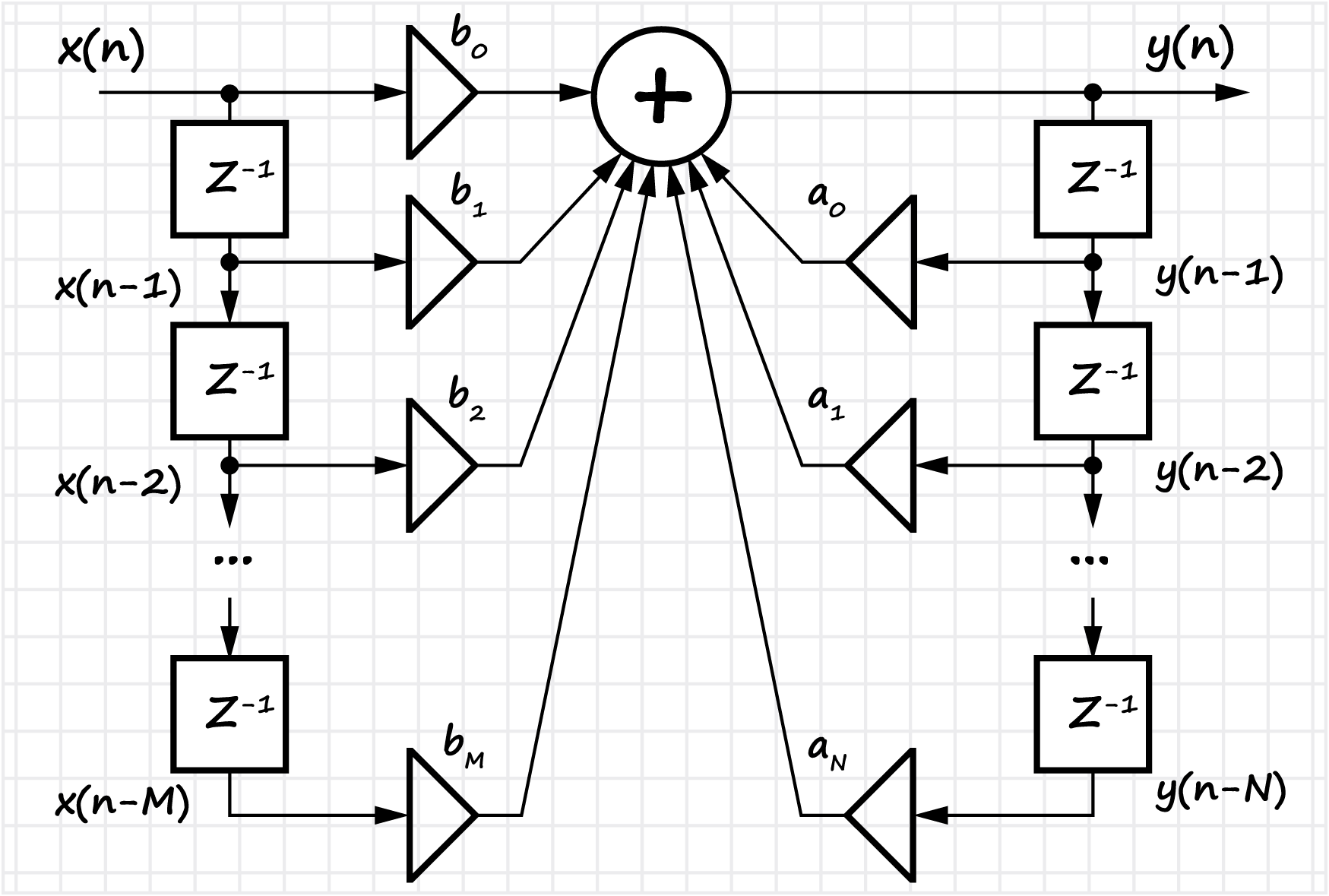
For FIR filters, the filter design process is shown from the stage of development of technical specifications (with the main parameters indicated), to software and hardware implementation - search for filter coefficients (taking into account the form of representation of the number, bit depth, etc.). The definitions of symmetric FIR filters, linear phase response and its relationship with the concept of group delay are introduced.

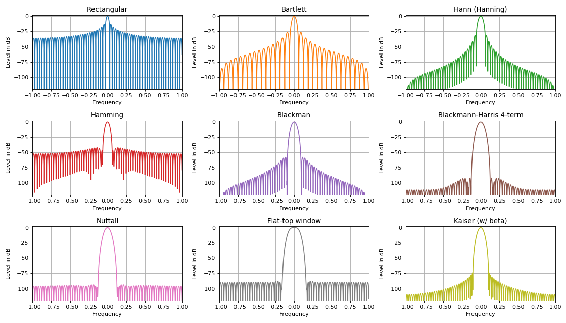
In the tasks of digital signal processing, window functions of various shapes are used, which, when superimposed on a signal in the time domain, can qualitatively improve its spectral characteristics. A large number of various windows is due primarily to one of the main features of any window overlay. This feature is expressed in the relationship between the level of the side lobes and the width of the central lobe. Rule:

One of the applications of window functions: detection of weak signals against the background of stronger ones by suppressing the level of side lobes. The main window functions in DSP tasks are ** triangular, sinusoidal, Lanczos, Hann, Hamming, Blackman, Harris, Blackman-Harris window, flat-top window, Natall, Gauss, Kaiser window ** and many others. Most of them are expressed through a finite series by summing harmonic signals with specific weights. Such signals are perfectly implemented in practice on any hardware devices (programmable logic circuits or signal processors).
This section discusses the issues of multi-speed signal processing - changes in the sampling frequency. Multi-speed processing of signals (multirate processing) suggests that in the process of linear conversion of digital signals, it is possible to change the sampling frequency in the direction of decreasing or increasing, or in a fractional number of times. This leads to more efficient signal processing, as it opens the possibility of using the minimum allowable sampling frequencies and, as a result, a significant reduction in the required computing performance of the designed digital system.
Decimation (decimation) - downsampling. Interpolation - increasing the sampling rate.
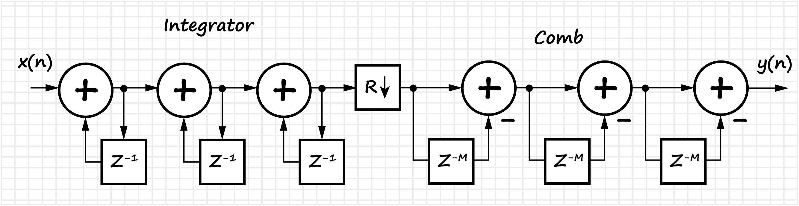
The section also considers the class of homogeneous FIR filters, which are called integral-comb filters (CIC, Cascaded integrator – comb). The implementation, basic properties and features of CIC filters are shown. Due to the linearity of the mathematical operations that occur in the CIC filter, it is possible to cascade several filters in a row, which gives a proportional decrease in the level of the side lobes, but also increases the “blockage” of the main lobe of the amplitude-frequency characteristic.
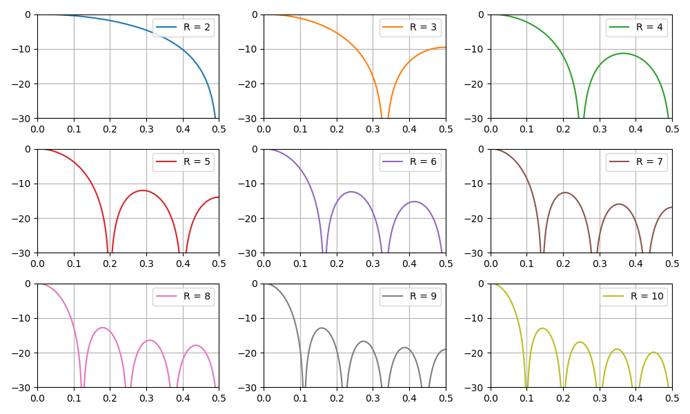
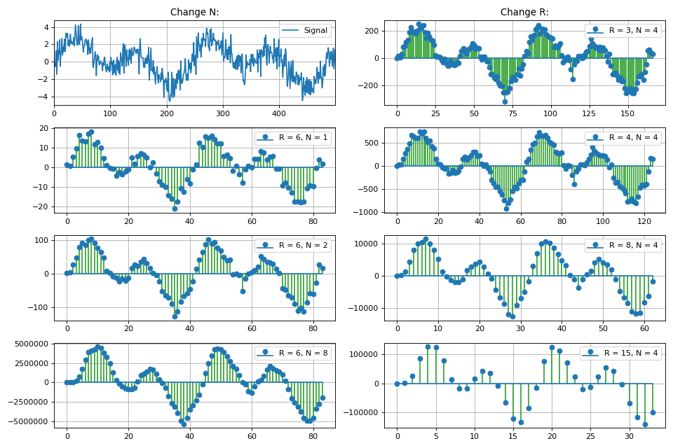
Graph of the frequency response of the filter depending on the decimation coefficient:
Also in this section we discuss the issue of increasing the bit depth of the data at the output of the CIC filter depending on its parameters. This is especially important in software implementation tasks, in particular on FPGAs.
For practical implementation of CIC filters in Python, a separate class CicFilter has been developed that implements decimation and interpolation methods. Also shown are sample rate changes using the built-in methods from the scipy Python package.
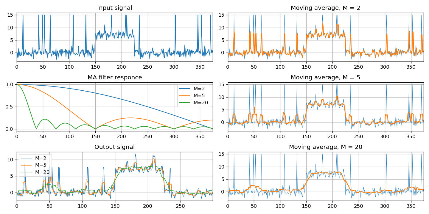
Finally, this section provides a special class of filters - the moving average. Three implementation methods are shown: through convolution of signals, using an FIR filter and an IIR filter.
I hope this lecture course in conjunction with my previous articles on digital FPGA signal processing will bring practical benefits and help the reader better understand the basics of digital signal processing. This project will be improved and supplemented with new useful and no less interesting material. Follow the development!
In addition to this material, I support and develop my project on the main DSP modules (in Python). It contains a package for generating various signals, a class of CIC filters for decimation and interpolation problems, an algorithm for calculating the coefficients of a correcting FIR filter, a moving average filter, an algorithm for calculating an ultra-long FFT through two-dimensional conversion methods (the latter was very useful when working with hardware implementation on FPGAs) .
Thanks for attention!
Often people turn to me with questions on tasks from the field of digital signal processing (DSP). I tell in detail the nuances, suggest the necessary sources of information. But all listeners, as time has shown, lack practical tasks and examples in the process of learning this area. In this regard, I decided to write a short interactive course on digital signal processing and put it in the public domain .
Most of the training material for visual and interactive presentation is implemented using the Jupyter Notebook . It is assumed that the reader has basic knowledge of the field of higher mathematics, as well as a little command of the Python programming language.
Lecture list
This course contains materials in the form of finished lectures on various topics from the field of digital signal processing. Materials are presented using Python libraries (numpy, scipy, matplotlib packages, etc.). The basic information for this course was taken from my lectures, which I, as a graduate student, gave to students of the Moscow Energy Institute (NRU MEI). Part of the information from these lectures was used at training seminars at the Center for Contemporary Electronics , where I acted as a lecturer. In addition, this material includes the translation of various scientific articles, compilation of information from reliable sources and literature on digital signal processing, as well as official documentation on application packages and built-in functions of the scipy and numpy libraries of Python.
For MATLAB (GNU Octave) users, mastering the material from the point of view of program code is not difficult, since the main functions and their attributes are largely identical and similar to the methods from the Python libraries.
All materials are grouped by the main topics of digital signal processing:
- Signals: analog, discrete, digital. Z conversion
- Fourier transform: amplitude and phase signal, DFT and FFT,
- Convolution and correlation. Linear and cyclic convolution. Quick convolution
- Random processes. White noise. Probability density function
- Deterministic signals. Modulation: AM, FM, FM, LFM. Manipulation
- Signal Filtering: IIR, FIR filters
- Window functions in filtering tasks. Detection of weak signals.
- Resampling: decimation and interpolation. CIC filters, moving average filters
The list of lectures is sufficient
Where to find?
All materials are absolutely free and available as an open repository on my github as an opensource project . Materials are presented in two formats - in the form of Jupyter Notebooks for interactive work, study and editing, and in the form of HTML files compiled from these notebooks (after downloading from the github they have a quite suitable format for reading and printing).
The following is a very brief description of the sections of the course with short explanations, terms and definitions. Basic information is available in the initial lectures, here is only a brief overview!
Signals. Z conversion
Introductory section, which contains basic information on the types of signals. The concept of a discrete sequence, delta function and Heaviside function (unit jump) is introduced.
All signals according to the method of presentation on the set can be divided into four groups:
- analog - are described by functions continuous in time,
- discrete - are interrupted in time with a step specified by sampling,
- quantized - have a set of finite levels (usually in amplitude),
- digital - a combination of the properties of discrete and quantized signals.
For the correct reconstruction of an analog signal from a digital one without distortion and loss, the sampling theorem known as the Kotelnikov (Nyquist-Shannon) theorem is used .
Any continuous signal with a limited spectrum can be restored uniquely and without loss by its discrete samples taken with a frequency strictly greater than twice the upper frequency of the spectrum of a continuous signal.
Such an interpretation is valid provided that the continuous function of time occupies a frequency band from 0 to the value of the upper frequency. If the quantization and discretization steps are chosen incorrectly, the signal will be distorted from analog to discrete.
Also in this section, the Z-transformation and its properties are described, and the representation of discrete sequences in the Z-form is shown.
Example of a finite discrete sequence:
x(nT) = {2, 1, -2, 0, 2, 3, 1, 0}An example of the same sequence in the Z-form:
X (z) = 2 + z -1 - 2z -2 + 2z -4 + 3z -5 + 1z -6
Fourier transform. Properties DFT and FFT
This section describes the concept of the time and frequency domain of a signal. The definition of the discrete Fourier transform (DFT) is introduced. The direct and inverse DFTs and their main properties are considered. Shown is the transition from the DFT to the fast Fourier transform (FFT) algorithm in base 2 (decimation algorithms in frequency and time). Reflected the effectiveness of FFT in comparison with DFT.
In particular, this section describes the Python package scipy.ffpack for computing various Fourier transforms (sine, cosine, direct, inverse, multidimensional, real).
The Fourier transform allows you to represent any function as a set of harmonic signals! The Fourier transform is the basis of convolution methods and the design of digital correlators, is actively used in spectral analysis, and is used when working with long numbers.
Features of the spectra of discrete signals:
1. The spectral density of a discrete signal is a periodic function with a period equal to the sampling frequency.
2. If the discrete sequence is real , then the spectral density modulus of such a sequence is an even function, and the argument is an odd frequency function.
Harmonic Signal Spectrum:
Comparison of the efficacy of DFT and FFT
The efficiency of the FFT algorithm and the number of operations performed linearly depends on the sequence length N:
| N | DFT | FFT | The ratio of the number of complex additions | The ratio of the number of complex multiplications | ||
|---|---|---|---|---|---|---|
| The number of multiplication operations | Number of addition operations | The number of multiplication operations | Number of addition operations | |||
| 2 | 4 | 2 | 1 | 2 | 4 | 1 |
| 4 | 16 | 12 | 4 | 8 | 4 | 1.5 |
| 8 | 64 | 56 | 12 | 24 | 5.3 | 2.3 |
| 16 | 256 | 240 | 32 | 64 | 8 | 3.75 |
| 32 | 1024 | 992 | 80 | 160 | 12.8 | 6.2 |
| 64 | 4096 | 4032 | 192 | 384 | 21.3 | 10.5 |
| 128 | 16384 | 16256 | 448 | 896 | 36.6 | 18.1 |
| ... | ... | ... | ... | ... | ... | ... |
| 4096 | 16777216 | 16773120 | 24576 | 49152 | 683 | 341 |
| 8192 | 67108864 | 67100672 | 53248 | 106496 | 1260 | 630 |
As you can see, the longer the conversion length, the greater the savings in computing resources (in terms of processing speed or the number of hardware units)!
Any arbitrary waveform can be represented as a set of harmonic signals of different frequencies. In other words, a signal of complex shape in the time domain has a set of complex samples in the frequency domain, which are called * harmonics *. These samples express the amplitude and phase of the harmonic effect at a specific frequency. The larger the set of harmonics in the frequency domain, the more accurately the complex waveform appears.
Convolution and correlation
This section introduces the concept of correlation and convolution for discrete random and deterministic sequences. The relationship between autocorrelation and cross-correlation functions with convolution is shown. The properties of convolution are described, in particular, the methods of linear and cyclic convolution of a discrete signal with detailed analysis on the example of a discrete sequence are considered. In addition, a method for computing “fast” convolution using FFT algorithms is shown.
In real problems, the question is often raised about the degree of similarity of one process to another or about the independence of one process from another. In other words, it is necessary to determine the relationship between the signals, that is, to find the correlation. Correlation methods are used in a wide range of tasks: signal search, computer vision and image processing, in radar problems to determine the characteristics of targets and determine the distance to an object. In addition, correlation is used to search for weak signals in noise.
The convolution describes the interaction of signals with each other. If one of the signals is the impulse response of the filter, then the convolution of the input sequence with the impulse response is nothing but a reaction of the circuit to the input action. In other words, the resulting signal reflects the passage of the signal through the filter.
Autocorrelation function(ACF) is used in coding information. The choice of the coding sequence according to the parameters of length, frequency and shape is largely due to the correlation properties of this sequence. The best code sequence has the lowest probability of false detection or operation (for detecting signals, for threshold devices) or false synchronization (for transmitting and receiving code sequences).
This section presents a table comparing the effectiveness of fast convolution and convolution calculated by the direct formula (by the number of real multiplications).
As you can see, for FFT lengths up to 64, fast convolution loseshave a direct method. However, with an increase in the FFT length, the results change in the opposite direction - a quick convolution begins to outperform the direct method. Obviously, the longer the FFT, the better the gain in the frequency method.
| N | Convolution | Quick convolution | Attitude |
|---|---|---|---|
| 8 | 64 | 448 | 0.14 |
| 16 | 256 | 1088 | 0.24 |
| 32 | 1024 | 2560 | 0.4 |
| 64 | 4096 | 5888 | 0.7 |
| 128 | 16K | 13312 | 1.23 |
| ... | ... | .. | ... |
| 2048 | 4M | 311296 | 13.5 |
Random Signals and Noise
In this section, the concept of random signals, probability density, random distribution law is introduced. Mathematical moments are considered - mean (mathematical expectation) and variance (or the root of this quantity is the standard deviation). Also in this section, the normal distribution and the related concept of white noise are considered as the main source of noise (interference) during signal processing.
A random signal is a function of time whose values are not known in advance and can only be predicted with some probability . The main characteristics of random signals include:
- distribution law (the relative residence time of the signal value in a certain interval),
- spectral distribution of signal power.
In DSP tasks, random signals are divided into two classes:
- noise - random fluctuations consisting of a set of different frequencies and amplitudes,
- signals carrying information, for the processing of which it is necessary to resort to probabilistic methods.
Using random variables, we can simulate the effect of a real medium on the passage of a signal from a source to a data receiver. When a signal passes through some noisy link, the so-called white noise is added to the signal. As a rule, the spectral density of such noise is uniformly (equally) distributed at all frequencies, and the noise values in the time domain are normally distributed (Gaussian distribution law). Since white noise is physically added to the signal amplitudes in the selected time samples, it is called Additive white Gaussian noise (AWGN).
Signals, Modulation and Manipulation
This section shows the basic methods for changing one or more parameters of a harmonic signal. The concepts of amplitude, frequency and phase modulation are introduced. In particular, the linear frequency modulation used in radar problems is highlighted. The main characteristics of the signals, the spectra of the modulated signals depending on the modulation parameters are shown.
For convenience, a set of functions has been created in Python that implements the above types of modulation. Example of chirp signal implementation:
def signal_chirp(amp=1.0, freq=0.0, beta=0.25, period=100, **kwargs):
    """
    Create Chirp signal
    Parameters
    ----------
    amp : float
        Signal magnitude
    beta : float
        Modulation bandwidth: beta < N for complex, beta < 0.5N for real
    freq : float or int
        Linear frequency of signal
    period : integer
        Number of points for signal (same as period)
    kwargs : bool
        Complex signal if is_complex = True
        Modulated by half-sine wave if is_modsine = True
    """
    is_complex = kwargs.get('is_complex', False)
    is_modsine = kwargs.get('is_modsine', False)
    t = np.linspace(0, 1, period)
    tt = np.pi * (freq * t + beta * t ** 2)
    if is_complex is True:
        res = amp * (np.cos(tt) + 1j * np.sin(tt))
    else:
        res = amp * np.cos(tt)
    if is_modsine is True:
        return res * np.sin(np.pi * t)
    return res
Also in this section from the theory of transmission of discrete messages types of digital modulation - manipulations are described. As in the case of analog signals, digital harmonic sequences can be manipulated in amplitude, phase and frequency (or several parameters at once).
Digital Filters - IIR and FIR
A sufficiently large section devoted to digital filtering of discrete sequences. In digital signal processing tasks, data flows through circuits called filters . Digital filters, like analog ones, have different characteristics - frequency: frequency response, phase response, time: impulse response, as well as the transfer characteristic of the filter. Digital filters are mainly used to improve signal quality — to isolate a signal from a data sequence, or to degrade unwanted signals — to suppress certain signals in incoming sample sequences.
The section lists the main advantages and disadvantages of digital filters (compared to analog). The concept of impulse and transfer characteristics of the filter is introduced. Two classes of filters are considered - with an infinite impulse response (IIR) and a finite impulse response (FIR). A method for designing filters in canonical and direct form is shown . For FIR filters, the question of how to switch to a recursive form is considered.
For FIR filters, the filter design process is shown from the stage of development of technical specifications (with the main parameters indicated), to software and hardware implementation - search for filter coefficients (taking into account the form of representation of the number, bit depth, etc.). The definitions of symmetric FIR filters, linear phase response and its relationship with the concept of group delay are introduced.
Window functions in filtering tasks
In the tasks of digital signal processing, window functions of various shapes are used, which, when superimposed on a signal in the time domain, can qualitatively improve its spectral characteristics. A large number of various windows is due primarily to one of the main features of any window overlay. This feature is expressed in the relationship between the level of the side lobes and the width of the central lobe. Rule:
The stronger the suppression of the side lobes of the spectrum, the wider the main lobe of the spectrum and vice versa.
One of the applications of window functions: detection of weak signals against the background of stronger ones by suppressing the level of side lobes. The main window functions in DSP tasks are ** triangular, sinusoidal, Lanczos, Hann, Hamming, Blackman, Harris, Blackman-Harris window, flat-top window, Natall, Gauss, Kaiser window ** and many others. Most of them are expressed through a finite series by summing harmonic signals with specific weights. Such signals are perfectly implemented in practice on any hardware devices (programmable logic circuits or signal processors).
Resampling. Decimation and interpolation
This section discusses the issues of multi-speed signal processing - changes in the sampling frequency. Multi-speed processing of signals (multirate processing) suggests that in the process of linear conversion of digital signals, it is possible to change the sampling frequency in the direction of decreasing or increasing, or in a fractional number of times. This leads to more efficient signal processing, as it opens the possibility of using the minimum allowable sampling frequencies and, as a result, a significant reduction in the required computing performance of the designed digital system.
Decimation (decimation) - downsampling. Interpolation - increasing the sampling rate.
The section also considers the class of homogeneous FIR filters, which are called integral-comb filters (CIC, Cascaded integrator – comb). The implementation, basic properties and features of CIC filters are shown. Due to the linearity of the mathematical operations that occur in the CIC filter, it is possible to cascade several filters in a row, which gives a proportional decrease in the level of the side lobes, but also increases the “blockage” of the main lobe of the amplitude-frequency characteristic.
Graph of the frequency response of the filter depending on the decimation coefficient:
Also in this section we discuss the issue of increasing the bit depth of the data at the output of the CIC filter depending on its parameters. This is especially important in software implementation tasks, in particular on FPGAs.
For practical implementation of CIC filters in Python, a separate class CicFilter has been developed that implements decimation and interpolation methods. Also shown are sample rate changes using the built-in methods from the scipy Python package.
Python CicFilter Class for Digital Signal Processing
class CicFilter:
    """
    Cascaded Integrator-Comb (CIC) filter is an optimized class of
    finite impulse response (FIR) filter.
    CIC filter combines an interpolator or decimator, so it has some
    parameters:
    R - decimation or interpolation ratio,
    N - number of stages in filter (or filter order)
    M - number of samples per stage (1 or 2)*
    * for this realisation of CIC filter just leave M = 1.
    CIC filter is used in multi-rate processing. In hardware
    applications CIC filter doesn't need multipliers, just only
    adders / subtractors and delay lines.
    Equation for 1st order CIC filter:
    y[n] = x[n] - x[n-RM] + y[n-1].
    Parameters
    ----------
    x : np.array
        input signal
    """
    def __init__(self, x):
        self.x = x
    def decimator(self, r, n):
        """
        CIC decimator: Integrator + Decimator + Comb
        Parameters
        ----------
        r : int
            decimation rate
        n : int
            filter order
        """
        # integrator
        y = self.x[:]
        for i in range(n):
            y = np.cumsum(y)
        # decimator
        y = y[::r]
        # comb stage
        return np.diff(y, n=n, prepend=np.zeros(n))
    def interpolator(self, r, n, mode=False):
        """
        CIC inteprolator: Comb + Decimator + Integrator
        Parameters
        ----------
        r : int
            interpolation rate
        n : int
            filter order
        mode : bool
            False - zero padding, True - value padding.
        """
        # comb stage
        y = np.diff(self.x, n=n,
                    prepend=np.zeros(n), append=np.zeros(n))
        # interpolation
        if mode:
            y = np.repeat(y, r)
        else:
            y = np.array([i if j == 0 else 0 for i in y for j in range(r)])
        # integrator
        for i in range(n):
            y = np.cumsum(y)
        if mode:
            return y[1:1 - n * r]
        else:
            return y[r - 1:-n * r + r - 1]
Finally, this section provides a special class of filters - the moving average. Three implementation methods are shown: through convolution of signals, using an FIR filter and an IIR filter.
Conclusion
I hope this lecture course in conjunction with my previous articles on digital FPGA signal processing will bring practical benefits and help the reader better understand the basics of digital signal processing. This project will be improved and supplemented with new useful and no less interesting material. Follow the development!
In addition to this material, I support and develop my project on the main DSP modules (in Python). It contains a package for generating various signals, a class of CIC filters for decimation and interpolation problems, an algorithm for calculating the coefficients of a correcting FIR filter, a moving average filter, an algorithm for calculating an ultra-long FFT through two-dimensional conversion methods (the latter was very useful when working with hardware implementation on FPGAs) .
Thanks for attention!