Dynamic programming in the real world: seam cutting
- Transfer
Dynamic programming has a reputation for the method that you study at the university, and then only remember during interviews. But in fact, the method is applicable in many situations. In fact, this is a technique for effectively solving problems that can be divided into many highly repetitive subtasks .
In the article I will show an interesting real application of dynamic programming - the seam carving task. The task and methodology are described in detail in the work of Avidan and Shamir “Cutting seams for resizing images based on content” (article in the public domain).
This is one of a series of articles on dynamic programming. If you want to brush up on methods, see the illustrated introduction to dynamic programming .
To solve a real problem using dynamic programming, you need to formulate it correctly. This section describes the necessary presets for the selected task.
The authors of the original article describe content-oriented image resizing, that is, changing the width or height of the image based on the content. See the original work for details, and I offer a brief overview. Suppose you want to resize a photo of a surfer:

Top view of a surfer in the middle of a calm ocean, with turbulent waves on the right. Photo: Kiril Dobrev on Pixabay
As described in detail in the article, there are several ways to reduce the image width: these are standard cropping and scaling, with their inherent disadvantages, as well as removing columns of pixels from the middle. As you can imagine, this leaves a visible seam in the photo, where the image on the left and right do not match. And in this way, you can delete only a limited amount of image.

An attempt to reduce the width by trimming the left side and cutting the block out of the middle. The latter leaves a visible seam.
Avidan and Shamir in the article describe the new technique of “seam carving”. It first identifies less important “low-energy” areas, and then calculates the low-energy “seams” that pass through the picture. In the case of reducing the width of the image, a vertical seam is determined from the top of the image to the bottom, which on each line is shifted to the left or right by no more than one pixel.
In the surfer’s photo, the lowest energy seam runs through the middle of the image, where the water is the quietest. This is consistent with our intuition.

The lowest-energy seam found in the image of the surfer is shown with a red line five pixels wide for visibility, although in fact the seam is only one pixel wide.
Having determined the seam with the least energy, and then removing it, we reduce the image width by one pixel. Repeating this process over and over again significantly reduces the width of the entire photo.

Image of a surfer after reducing the width by 1024 pixels.
Again, the algorithm logically removed the still water in the middle, as well as on the left side of the photo. But unlike cropping, the texture of the water on the left is preserved and there are no sharp transitions. True, you can find some imperfect transitions in the center, but basically the result looks natural.
The magic is to find the lowest energy seam. To do this, we first assign energy to each pixel in the image. Then we use dynamic programming to find the path through the image with the least energy - this algorithm will be discussed in detail in the next section. First, let's look at how to assign pixels energy values.
The scientific article discusses several energy functions and their differences. Let's not complicate it and take a function that simply captures the amount of color change around each pixel. To complete the picture, I will describe the energy function in more detail in case you want to implement it yourself, but this is just a preset for subsequent dynamic programming calculations.

On the left are three pixels from dark to light. The difference between the first and last is great. On the right are three dark pixels with a small difference in color intensity.
To calculate the energy of a particular pixel, look at the pixels to the left and right of it. Component-wise, we compute the square of the distance between them, that is, the square of the difference between the red, green, and blue components, and then add them. We do the same for pixels above and below the center. Finally, add up the horizontal and vertical distances.
The only caveat - say, if a pixel is on the left edge, then there is no neighbor on the left. In this case, we compare only with the right pixel. Similar checks are performed for pixels at the upper, right, and lower edges.
The energy function is great if the neighboring pixels are very different in color, and small if they are similar.
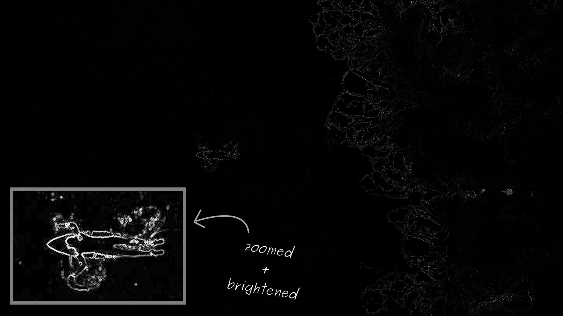
The energy of each pixel in a surfer’s photo: the lighter - the higher it is. As expected, the surfer has the highest energy in the middle and turbulent waves on the right
The energy function works well on a surfer photo. However, it takes a very wide range of values. Therefore, when rendering, it seems that in most of the photos pixels have zero energy. In fact, there are simply very low values compared to the regions with the highest energy. To simplify the visualization, I zoomed in the surfer and highlighted this area.
By calculating the energy of each pixel, we can find the seam with the lowest energy from the top of the image to the bottom. The same analysis applies to horizontal seams to reduce the height of the original image. However, we will focus on vertical ones.
Let's start with the definition:
It is important to note that the joint with the lowest energy does not necessarily go through all the pixels with the lowest energy. The total energy of all, not individual pixels, is taken into account.

The greedy approach does not work. Choosing a low-energy pixel at an early stage, we get stuck in the high-energy region of the image (the red path on the right).
As you can see, you can’t just select the lowest-energy pixel in the next line.
The problem with the greedy approach is that when deciding on the next step, we do not take into account the rest of the seam ahead. We cannot look into the future, but we are able to take into account everything that we already know by now.
Let's turn the task upside down. Instead of choosing between several pixels to continue one seam, we will choose between several seams to go to one pixel . What we need to do is take each pixel and choose between the pixels in the line above, from which the seam can come. If each of the pixels in the line above encodes the path traveled to this point, then we are essentially looking at the full history to this point.

For each pixel, we study three pixels in the line above. Fundamental choice - which of the seams to continue?
This assumes a subtask for each pixel in the image. The subtask should find the best path to a specific pixel, so it’s a good idea to associate with each pixel the energy of the low-energy seam that ends in that pixel .
Unlike the greedy approach, the above approach essentially tries all possible paths through the image. It’s just that when checking all possible paths, the same subtasks are solved again and again, which makes this approach an ideal option for dynamic programming.
As usual, now we need to formalize the idea in a recursive relation. There is a subtask corresponding to each pixel in the original image, so the inputs to our recurrence relation can be just coordinates and
and  of this pixel. This provides integer inputs, making it easy to organize subtasks, as well as the ability to store previously calculated values in a two-dimensional array.
Define a function , which represents the energy of the vertical seam with the least energy. It starts at the top of the image and ends in a pixel
 . Title
 selected as in the original scientific article.
First, you need a basic version. All seams that end on the top line have a length of only one pixel. Thus, a seam with minimum energy is just a pixel with minimum energy:
For pixels in the remaining rows, look at the pixels at the top. Since the seam should be continuous, we take into account only three pixels located at the top left, top and top right. From them we select the seam with the lowest energy, which ends in one of these pixels, and add the energy of the current pixel:
As a borderline situation, consider the case when the current pixel is at the left or right edge of the image. In these cases, we omit for pixels on the left edge or
  on the right edge.
Finally, you need to extract the energy of the low-energy seam, which covers the entire height of the image. This means that we look at the bottom line of the image and select the lowest-energy seam that ends at one of these pixels. For photo wide and tall
  pixels:
So, we got a recurrence relation with all the necessary properties:
Since each subtaskcorresponds to one pixel of the original image, the dependency graph is very easy to visualize. Just place them on a two-dimensional grid, as in the original image!
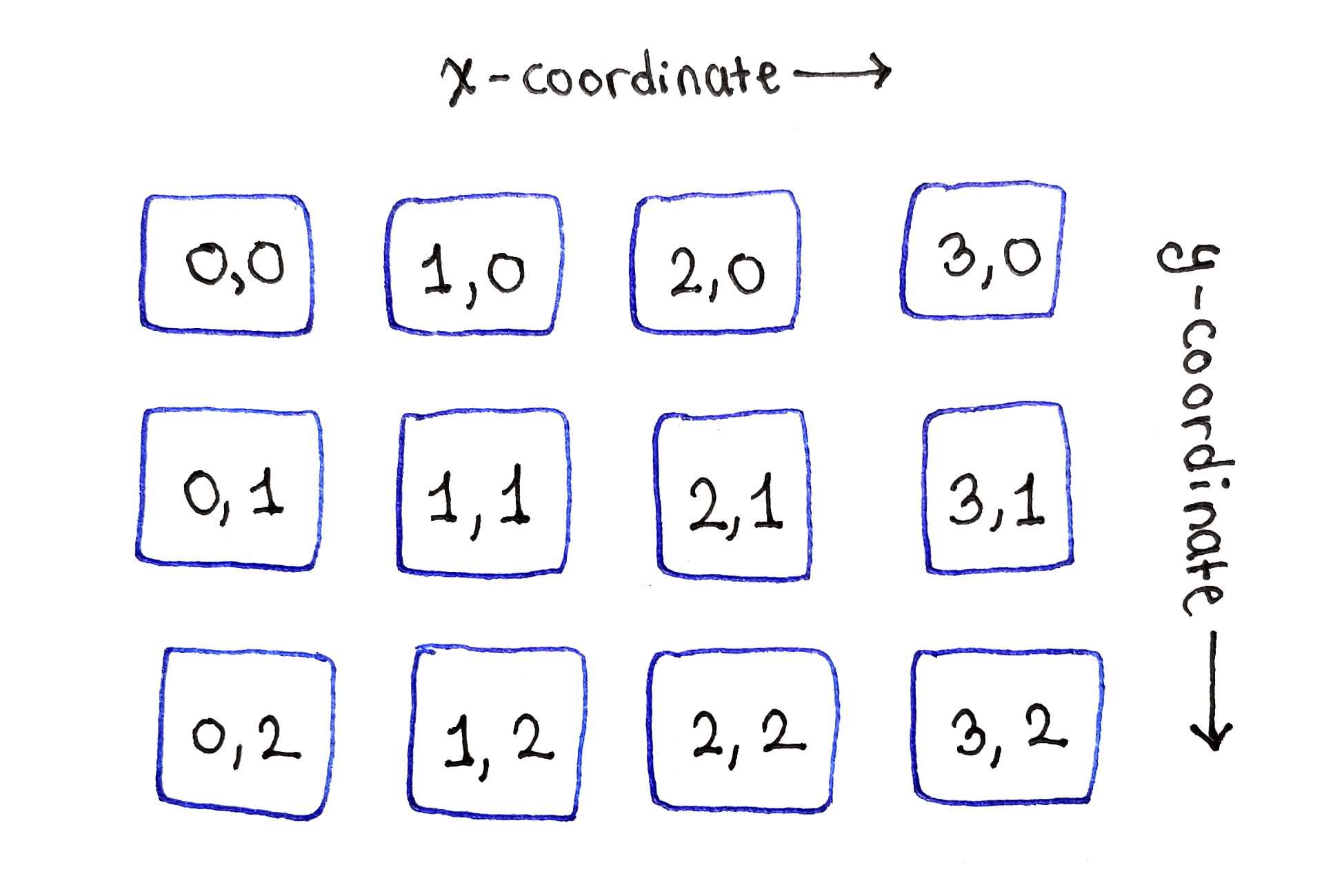
The subtasks are located in a two-dimensional grid, as are the pixels in the original image.
As follows from the base scenario of the recurrence relation, the top row of subtasks can be initialized with the energy values of individual pixels.

The top row is independent of other subtasks. Note the absence of arrows from the top row of cells.
In the second line, dependencies begin to appear. Firstly, in the leftmost cell in the second row we are faced with a border situation. Since there are no cells on the left, the cell depends only on the cells located directly above it and on the upper right. The same thing will happen later with the leftmost cell in the third row.

The subtasks on the left edge depend on only two subtasks above them.
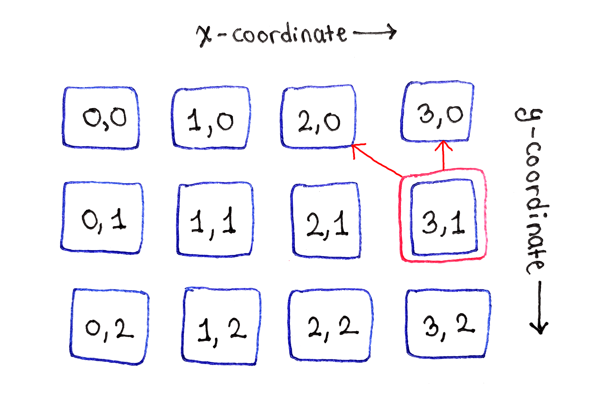
In the second cell of the second row (1,1), we see the most typical manifestation of the recurrence relation. This cell depends on three cells: top left, right above it and top right. This dependency structure applies to all “middle” cells in the second and subsequent rows.

The subtasks between the left and right edges depend on three subtasks from above.
Finally, the cell on the right edge represents the second boundary situation. Since there are no more cells on the right, it depends only on the cells directly at the top and top left.
The subtasks on the right edge depend on only two cells on top.
The process is repeated for all subsequent lines.

Since there are many arrows in the dependency graph, this animation shows the dependencies for each subtask in turn. The
full dependency graph scares a lot of arrows, but looking at them one at a time helps to establish explicit patterns.
After conducting this analysis, we got the processing order:
Since each row depends only on the previous one, you need to save only two rows of data: one for the previous row and one for the current row. Moving from left to right, we can even discard individual elements from the previous row as they are used. However, this complicates the algorithm, as it will have to figure out which parts of the previous line can be discarded.
In the following Python code, the input is a list of lines, where each line contains a list of numbers representing the individual pixel energies in that line. The input is called.
Let's start by calculating the energy of the seams of the upper row, simply by copying the individual pixel energies in the upper row:
Then we cycle through the remaining input lines, calculating the seam energies for each line. The most “difficult” part is to determine which elements of the previous line to refer to, since there are no pixels to the left of the left edge or to the right of the right edge.
At each iteration, a new list of seam energies for the current line is created. At the end of the iteration, we replace the data of the previous line with the data of the current line for the next iteration. This is how we discard the previous line:
The
You can test this implementation by wrapping the code in a function, and then calling it with the two-dimensional array that you built. The following input has been chosen so that the greedy approach fails, with an obvious seam with the lowest energy:
Each pixel in the original image corresponds to one subtask. For each of the subtasks, there are no more than three dependencies, so solving each of them involves a constant amount of work. The last row is held twice. So for image wide and tall pixels time complexity is  .
.
At each moment in time, we have two lists: one for the previous line and one for the current. In the first elements, and the second gradually increases to . Thus, the spatial complexity is equal to that is just
  .
.
Note that if we actually discarded the data elements of the previous row, we would shorten the list of elements of the previous row at about the same speed as the list of the current row grows. Thus spatial complexity will remain. Although the width may vary, this is usually not so important.
So, we found the meaning of the low-energy seam, but what to do with this information? After all, in fact, we are not concerned about the importance of energy, but the seam itself! The problem is that there is no way from the final pixel to return to the rest of the seam.
This is what I missed in previous articles, but the same applies to many dynamic programming issues. For example, if you remember the task of a house robber , we found the maximum value for the amount of robbery, but not which specific houses need to be robbed to obtain this amount.
General answer: store back pointers . In the task of cutting seams, we need not only the value of the energy of the seam at each pixel. You also need to know which of the pixels in the previous row led to this energy. By storing this information, we can follow the reverse pointers right up to the top line, getting the coordinates of all the pixels that make up the joint with the least energy.
First, create a class for storing energy and back pointers. Energy will be used to calculate subtasks. Since the backward pointer determines which pixel in the previous line gave the current energy, we can imagine it simply as the x coordinate.
The calculation result for each subtask will be not just a number, but an instance of this class.
In the end, you need to go back along the entire height of the image, following the reverse signs to restore the seam with the least energy. Unfortunately, this means that you need to store pointers for all pixels in the image, not just the previous line.
To do this, we simply save the full result of all the subtasks, although it is technically possible to abandon the numerical energies of the seam of the previous lines. The results are stored in a two-dimensional array, which looks the same as the input array.
Let's start with the first line, which contains only individual pixel energies. Since there is no previous line, all the back pointers are missing, but for consistency we will still keep instances
The main loop works basically the same as the previous implementation, with the following differences:
Now the whole table of subtasks is filled and we can restore the seam with the least energy. We start by looking for the x coordinate in the bottom line, which corresponds to the joint with the least energy:
Now go from the bottom of the image to the top, changingfrom to the list representing our seam, and then set the value for the object pointed to
So the seam is built upward, the list can then be read in reverse order, if you need coordinates from top to bottom.
The time complexity is similar to the previous one, because we still need to process each pixel once. After looking at the last line and finding the joint with the least energy, we then go up the entire height of the image to restore the joint. So for the image time complexity equals
  .
.
As for the volume, we still keep a constant amount of data for each subtask, but now we do not discard any data. So we use volume .
.
As soon as the vertical joint with the lowest energy is found, we can simply copy the pixels from the original image to a new one. Each line of the new image contains all the pixels from the corresponding line of the original image, with the exception of the pixel from the seam with the lowest energy. Since we delete one pixel in each row, starting from the imagethen we get the image  .
.
We can repeat this process by recounting the energy function in the new image and finding the lowest-energy seam on it. It seems tempting to find more than one low-energy seam in the original image, and then delete them all at once. The problem is that the two seams can intersect. When the first one is deleted, the second one will become invalid because one or more pixels are missing from it.
Animation of the seam removal process. It is better to watch in full-screen mode for a clearer view of seams.
Each video frame is an image at each iteration with superimposed visualization of the seam with the least energy.
The article had a lot of detailed explanations, so let's end with a series of beautiful photos! The following photo shows a rock formation in Arches National Park: A

rock formation with a hole in Arches National Park. Photo: Mike Goad on Flickr
Energy feature for this image: The

energy of each pixel in the photo: the lighter the higher. Pay attention to the high energy around the edge of the hole.
The result of the calculation is such a seam with the lowest energy. Note that it passes through the rock on the right, entering directly into the rock formation where the illuminated part at the top of the rock matches the color of the sky. Perhaps you should choose a better energy function!

The lowest-energy seam found in the image is shown with a red line five pixels wide for visibility, although in reality the seam is only one pixel wide.
Finally, the image of the arch after resizing:

Arch after compression by 1024 pixels
The result is definitely not perfect: many edges of the mountain from The original image is distorted. One of the improvements may be the implementation of one of the other energy functions listed in the scientific article.
Although dynamic programming is usually discussed in theory, it is a useful practical method for solving complex problems. In this article, we examined one of the applications of dynamic programming: resizing images to fit content by cutting seams.
We applied the same principles of dividing a problem into smaller subtasks, analyzing the dependencies between these subtasks, and then solving the subtasks in an order that minimizes the spatial and temporal complexity of the algorithm. In addition, we studied the use of reverse pointers to not only find the energy value for the optimal seam, but also to determine the coordinates of each pixel that made up this value. Then we applied these parts to a real problem, which requires some pre- and post-processing for truly effective use of the dynamic programming algorithm.
In the article I will show an interesting real application of dynamic programming - the seam carving task. The task and methodology are described in detail in the work of Avidan and Shamir “Cutting seams for resizing images based on content” (article in the public domain).
This is one of a series of articles on dynamic programming. If you want to brush up on methods, see the illustrated introduction to dynamic programming .
Resize image based on content
To solve a real problem using dynamic programming, you need to formulate it correctly. This section describes the necessary presets for the selected task.
The authors of the original article describe content-oriented image resizing, that is, changing the width or height of the image based on the content. See the original work for details, and I offer a brief overview. Suppose you want to resize a photo of a surfer:
Top view of a surfer in the middle of a calm ocean, with turbulent waves on the right. Photo: Kiril Dobrev on Pixabay
As described in detail in the article, there are several ways to reduce the image width: these are standard cropping and scaling, with their inherent disadvantages, as well as removing columns of pixels from the middle. As you can imagine, this leaves a visible seam in the photo, where the image on the left and right do not match. And in this way, you can delete only a limited amount of image.
An attempt to reduce the width by trimming the left side and cutting the block out of the middle. The latter leaves a visible seam.
Avidan and Shamir in the article describe the new technique of “seam carving”. It first identifies less important “low-energy” areas, and then calculates the low-energy “seams” that pass through the picture. In the case of reducing the width of the image, a vertical seam is determined from the top of the image to the bottom, which on each line is shifted to the left or right by no more than one pixel.
In the surfer’s photo, the lowest energy seam runs through the middle of the image, where the water is the quietest. This is consistent with our intuition.
The lowest-energy seam found in the image of the surfer is shown with a red line five pixels wide for visibility, although in fact the seam is only one pixel wide.
Having determined the seam with the least energy, and then removing it, we reduce the image width by one pixel. Repeating this process over and over again significantly reduces the width of the entire photo.
Image of a surfer after reducing the width by 1024 pixels.
Again, the algorithm logically removed the still water in the middle, as well as on the left side of the photo. But unlike cropping, the texture of the water on the left is preserved and there are no sharp transitions. True, you can find some imperfect transitions in the center, but basically the result looks natural.
Image Energy Definition
The magic is to find the lowest energy seam. To do this, we first assign energy to each pixel in the image. Then we use dynamic programming to find the path through the image with the least energy - this algorithm will be discussed in detail in the next section. First, let's look at how to assign pixels energy values.
The scientific article discusses several energy functions and their differences. Let's not complicate it and take a function that simply captures the amount of color change around each pixel. To complete the picture, I will describe the energy function in more detail in case you want to implement it yourself, but this is just a preset for subsequent dynamic programming calculations.
On the left are three pixels from dark to light. The difference between the first and last is great. On the right are three dark pixels with a small difference in color intensity.
To calculate the energy of a particular pixel, look at the pixels to the left and right of it. Component-wise, we compute the square of the distance between them, that is, the square of the difference between the red, green, and blue components, and then add them. We do the same for pixels above and below the center. Finally, add up the horizontal and vertical distances.


The only caveat - say, if a pixel is on the left edge, then there is no neighbor on the left. In this case, we compare only with the right pixel. Similar checks are performed for pixels at the upper, right, and lower edges.
The energy function is great if the neighboring pixels are very different in color, and small if they are similar.
The energy of each pixel in a surfer’s photo: the lighter - the higher it is. As expected, the surfer has the highest energy in the middle and turbulent waves on the right
The energy function works well on a surfer photo. However, it takes a very wide range of values. Therefore, when rendering, it seems that in most of the photos pixels have zero energy. In fact, there are simply very low values compared to the regions with the highest energy. To simplify the visualization, I zoomed in the surfer and highlighted this area.
Search for low-energy seams with dynamic programming
By calculating the energy of each pixel, we can find the seam with the lowest energy from the top of the image to the bottom. The same analysis applies to horizontal seams to reduce the height of the original image. However, we will focus on vertical ones.
Let's start with the definition:
- A seam is a sequence of pixels, one pixel per line. The requirement is that between two consecutive lines the coordinatechanges by no more than one pixel. This preserves the seam sequence.
- The seam with the lowest energy is the one whose total energy over all pixels in the seam is minimized.
It is important to note that the joint with the lowest energy does not necessarily go through all the pixels with the lowest energy. The total energy of all, not individual pixels, is taken into account.
The greedy approach does not work. Choosing a low-energy pixel at an early stage, we get stuck in the high-energy region of the image (the red path on the right).
As you can see, you can’t just select the lowest-energy pixel in the next line.
We break the problem into subtasks
The problem with the greedy approach is that when deciding on the next step, we do not take into account the rest of the seam ahead. We cannot look into the future, but we are able to take into account everything that we already know by now.
Let's turn the task upside down. Instead of choosing between several pixels to continue one seam, we will choose between several seams to go to one pixel . What we need to do is take each pixel and choose between the pixels in the line above, from which the seam can come. If each of the pixels in the line above encodes the path traveled to this point, then we are essentially looking at the full history to this point.
For each pixel, we study three pixels in the line above. Fundamental choice - which of the seams to continue?
This assumes a subtask for each pixel in the image. The subtask should find the best path to a specific pixel, so it’s a good idea to associate with each pixel the energy of the low-energy seam that ends in that pixel .
Unlike the greedy approach, the above approach essentially tries all possible paths through the image. It’s just that when checking all possible paths, the same subtasks are solved again and again, which makes this approach an ideal option for dynamic programming.
Definition of a recurrence relation
As usual, now we need to formalize the idea in a recursive relation. There is a subtask corresponding to each pixel in the original image, so the inputs to our recurrence relation can be just coordinates
and of this pixel. This provides integer inputs, making it easy to organize subtasks, as well as the ability to store previously calculated values in a two-dimensional array. Define a function
, which represents the energy of the vertical seam with the least energy. It starts at the top of the image and ends in a pixel. Titleselected as in the original scientific article. First, you need a basic version. All seams that end on the top line have a length of only one pixel. Thus, a seam with minimum energy is just a pixel with minimum energy:

For pixels in the remaining rows, look at the pixels at the top. Since the seam should be continuous, we take into account only three pixels located at the top left, top and top right. From them we select the seam with the lowest energy, which ends in one of these pixels, and add the energy of the current pixel:

As a borderline situation, consider the case when the current pixel is at the left or right edge of the image. In these cases, we omit
for pixels on the left edge or on the right edge. Finally, you need to extract the energy of the low-energy seam, which covers the entire height of the image. This means that we look at the bottom line of the image and select the lowest-energy seam that ends at one of these pixels. For photo wide
and tall pixels:
So, we got a recurrence relation with all the necessary properties:
- A recurrence relation has integer inputs.
- The final answer is easy to extract from the relation.
- The ratio depends on oneself.
Verification of the DAG subtask (oriented acyclic graph)
Since each subtask
corresponds to one pixel of the original image, the dependency graph is very easy to visualize. Just place them on a two-dimensional grid, as in the original image! The subtasks are located in a two-dimensional grid, as are the pixels in the original image.
As follows from the base scenario of the recurrence relation, the top row of subtasks can be initialized with the energy values of individual pixels.
The top row is independent of other subtasks. Note the absence of arrows from the top row of cells.
In the second line, dependencies begin to appear. Firstly, in the leftmost cell in the second row we are faced with a border situation. Since there are no cells on the left, the cell
depends only on the cells located directly above it and on the upper right. The same thing will happen later with the leftmost cell in the third row. The subtasks on the left edge depend on only two subtasks above them.
In the second cell of the second row (1,1), we see the most typical manifestation of the recurrence relation. This cell depends on three cells: top left, right above it and top right. This dependency structure applies to all “middle” cells in the second and subsequent rows.
The subtasks between the left and right edges depend on three subtasks from above.
Finally, the cell on the right edge represents the second boundary situation. Since there are no more cells on the right, it depends only on the cells directly at the top and top left.
The subtasks on the right edge depend on only two cells on top.
The process is repeated for all subsequent lines.
Since there are many arrows in the dependency graph, this animation shows the dependencies for each subtask in turn. The
full dependency graph scares a lot of arrows, but looking at them one at a time helps to establish explicit patterns.
Bottom up implementation
After conducting this analysis, we got the processing order:
- Go from the top of the image to the bottom.
- Each line can act in any order. The natural choice is to go from left to right.
Since each row depends only on the previous one, you need to save only two rows of data: one for the previous row and one for the current row. Moving from left to right, we can even discard individual elements from the previous row as they are used. However, this complicates the algorithm, as it will have to figure out which parts of the previous line can be discarded.
In the following Python code, the input is a list of lines, where each line contains a list of numbers representing the individual pixel energies in that line. The input is called
pixel_energies, and pixel_energies[y][x]represents the pixel energy in coordinates. Let's start by calculating the energy of the seams of the upper row, simply by copying the individual pixel energies in the upper row:
previous_seam_energies_row = list(pixel_energies[0])Then we cycle through the remaining input lines, calculating the seam energies for each line. The most “difficult” part is to determine which elements of the previous line to refer to, since there are no pixels to the left of the left edge or to the right of the right edge.
At each iteration, a new list of seam energies for the current line is created. At the end of the iteration, we replace the data of the previous line with the data of the current line for the next iteration. This is how we discard the previous line:
# Skip the first row in the following loop.
for y in range(1, len(pixel_energies)):
    pixel_energies_row = pixel_energies[y]
    seam_energies_row = []
    for x, pixel_energy in enumerate(pixel_energies_row):
        # Determine the range of x values to iterate over in the previous
        # row. The range depends on if the current pixel is in the middle of
        # the image, or on one of the edges.
        x_left = max(x - 1, 0)
        x_right = min(x + 1, len(pixel_energies_row) - 1)
        x_range = range(x_left, x_right + 1)
        min_seam_energy = pixel_energy + \
            min(previous_seam_energies_row[x_i] for x_i in x_range)
        seam_energies_row.append(min_seam_energy)
    previous_seam_energies_row = seam_energies_row
The
previous_seam_energies_rowbottom line contains the seam energy for the bottom line. We find the minimum value in this list - and this is the answer!min(seam_energy for seam_energy in previous_seam_energies_row)You can test this implementation by wrapping the code in a function, and then calling it with the two-dimensional array that you built. The following input has been chosen so that the greedy approach fails, with an obvious seam with the lowest energy:
ENERGIES = [
    [9, 9, 0, 9, 9],
    [9, 1, 9, 8, 9],
    [9, 9, 9, 9, 0],
    [9, 9, 9, 0, 9],
]
print(min_seam_energy(ENERGIES))
Spatial and temporal complexity
Each pixel in the original image corresponds to one subtask. For each of the subtasks, there are no more than three dependencies, so solving each of them involves a constant amount of work. The last row is held twice. So for image wide
and tall pixels time complexity is . At each moment in time, we have two lists: one for the previous line and one for the current. In the first
elements, and the second gradually increases to . Thus, the spatial complexity is equal tothat is just . Note that if we actually discarded the data elements of the previous row, we would shorten the list of elements of the previous row at about the same speed as the list of the current row grows. Thus spatial complexity will remain
. Although the width may vary, this is usually not so important.Low Energy Backward Pointers
So, we found the meaning of the low-energy seam, but what to do with this information? After all, in fact, we are not concerned about the importance of energy, but the seam itself! The problem is that there is no way from the final pixel to return to the rest of the seam.
This is what I missed in previous articles, but the same applies to many dynamic programming issues. For example, if you remember the task of a house robber , we found the maximum value for the amount of robbery, but not which specific houses need to be robbed to obtain this amount.
Representation of back pointers
General answer: store back pointers . In the task of cutting seams, we need not only the value of the energy of the seam at each pixel. You also need to know which of the pixels in the previous row led to this energy. By storing this information, we can follow the reverse pointers right up to the top line, getting the coordinates of all the pixels that make up the joint with the least energy.
First, create a class for storing energy and back pointers. Energy will be used to calculate subtasks. Since the backward pointer determines which pixel in the previous line gave the current energy, we can imagine it simply as the x coordinate.
class SeamEnergyWithBackPointer():
    def __init__(self, energy, x_coordinate_in_previous_row=None):
        self.energy = energy
        self.x_coordinate_in_previous_row = x_coordinate_in_previous_row
The calculation result for each subtask will be not just a number, but an instance of this class.
Backward Pointer Storage
In the end, you need to go back along the entire height of the image, following the reverse signs to restore the seam with the least energy. Unfortunately, this means that you need to store pointers for all pixels in the image, not just the previous line.
To do this, we simply save the full result of all the subtasks, although it is technically possible to abandon the numerical energies of the seam of the previous lines. The results are stored in a two-dimensional array, which looks the same as the input array.
Let's start with the first line, which contains only individual pixel energies. Since there is no previous line, all the back pointers are missing, but for consistency we will still keep instances
SeamEnergyWithBackPointers:seam_energies = []
# Initialize the top row of seam energies by copying over the top row of
# the pixel energies. There are no back pointers in the top row.
seam_energies.append([
SeamEnergyWithBackPointer(pixel_energy)
for pixel_energy in pixel_energies[0]
])The main loop works basically the same as the previous implementation, with the following differences:
- The data for the previous row contains instances
SeamEnergyWithBackPointer, so when calculating the value of the recurrence ratio, you should look for the energy of the seam inside these objects. - Saving data for the current pixel, you need to build a new instance
SeamEnergyWithBackPointer. Here we will store the seam energy for the current pixel, as well as the x coordinate from the previous line, used to calculate the current seam energy. - At the end of each row, instead of discarding the data of the previous row, we simply add the data of the current row to
seam_energies.
# Skip the first row in the following loop.
for y in range(1, len(pixel_energies)):
    pixel_energies_row = pixel_energies[y]
    seam_energies_row = []
    for x, pixel_energy in enumerate(pixel_energies_row):
        # Determine the range of x values to iterate over in the previous
        # row. The range depends on if the current pixel is in the middle of
        # the image, or on one of the edges.
        x_left = max(x - 1, 0)
        x_right = min(x + 1, len(pixel_energies_row) - 1)
        x_range = range(x_left, x_right + 1)
        min_parent_x = min(
            x_range,
            key=lambda x_i: seam_energies[y - 1][x_i].energy
        )
        min_seam_energy = SeamEnergyWithBackPointer(
            pixel_energy + seam_energies[y - 1][min_parent_x].energy,
            min_parent_x
        )
        seam_energies_row.append(min_seam_energy)
    seam_energies.append(seam_energies_row)
Follow the signs
Now the whole table of subtasks is filled and we can restore the seam with the least energy. We start by looking for the x coordinate in the bottom line, which corresponds to the joint with the least energy:
# Find the x coordinate with minimal seam energy in the bottom row.
min_seam_end_x = min(
    range(len(seam_energies[-1])),
    key=lambda x: seam_energies[-1][x].energy
)
Now go from the bottom of the image to the top, changing
from len(seam_energies) - 1to zero. At each iteration, add the current pair to the list representing our seam, and then set the value for the object pointed to SeamEnergyWithBackPointerin the current line.# Follow the back pointers to form a list of coordinates that form the
# lowest-energy seam.
seam = []
seam_point_x = min_seam_end_x
for y in range(len(seam_energies) - 1, -1, -1):
seam.append((seam_point_x, y))
seam_point_x = \
seam_energies[y][seam_point_x].x_coordinate_in_previous_row
seam.reverse()So the seam is built upward, the list can then be read in reverse order, if you need coordinates from top to bottom.
Spatial and temporal complexity
The time complexity is similar to the previous one, because we still need to process each pixel once. After looking at the last line and finding the joint with the least energy, we then go up the entire height of the image to restore the joint. So for the image
time complexity equals . As for the volume, we still keep a constant amount of data for each subtask, but now we do not discard any data. So we use volume
.Low energy seam removal
As soon as the vertical joint with the lowest energy is found, we can simply copy the pixels from the original image to a new one. Each line of the new image contains all the pixels from the corresponding line of the original image, with the exception of the pixel from the seam with the lowest energy. Since we delete one pixel in each row, starting from the image
then we get the image . We can repeat this process by recounting the energy function in the new image and finding the lowest-energy seam on it. It seems tempting to find more than one low-energy seam in the original image, and then delete them all at once. The problem is that the two seams can intersect. When the first one is deleted, the second one will become invalid because one or more pixels are missing from it.
Animation of the seam removal process. It is better to watch in full-screen mode for a clearer view of seams.
Each video frame is an image at each iteration with superimposed visualization of the seam with the least energy.
Another example
The article had a lot of detailed explanations, so let's end with a series of beautiful photos! The following photo shows a rock formation in Arches National Park: A
rock formation with a hole in Arches National Park. Photo: Mike Goad on Flickr
Energy feature for this image: The
energy of each pixel in the photo: the lighter the higher. Pay attention to the high energy around the edge of the hole.
The result of the calculation is such a seam with the lowest energy. Note that it passes through the rock on the right, entering directly into the rock formation where the illuminated part at the top of the rock matches the color of the sky. Perhaps you should choose a better energy function!
The lowest-energy seam found in the image is shown with a red line five pixels wide for visibility, although in reality the seam is only one pixel wide.
Finally, the image of the arch after resizing:
Arch after compression by 1024 pixels
The result is definitely not perfect: many edges of the mountain from The original image is distorted. One of the improvements may be the implementation of one of the other energy functions listed in the scientific article.
Although dynamic programming is usually discussed in theory, it is a useful practical method for solving complex problems. In this article, we examined one of the applications of dynamic programming: resizing images to fit content by cutting seams.
We applied the same principles of dividing a problem into smaller subtasks, analyzing the dependencies between these subtasks, and then solving the subtasks in an order that minimizes the spatial and temporal complexity of the algorithm. In addition, we studied the use of reverse pointers to not only find the energy value for the optimal seam, but also to determine the coordinates of each pixel that made up this value. Then we applied these parts to a real problem, which requires some pre- and post-processing for truly effective use of the dynamic programming algorithm.