July 1, 2019 at 15:52
The symmetry property of the cointegration relation
The purpose of this article is to share paradoxical results in the study of co-integration of time series : if the time series co-integrated with nearby
  , row not always co-integrated with a number .
If we study cointegration purely theoretically, then it is easy to prove that if the series co-integrated with then row co-integrated with . However, if we begin to study cointegration empirically, it turns out that theoretical calculations are not always confirmed. Why it happens?
Attitude called symmetric if  where
where  - the inverse ratio defined by the condition:
  tantamount to
  . In other words, if the relation
 then the relation .
Consider two a number of
  and
and  ,
,  . Cointegration is symmetric if
 entails
  that is, if the presence of direct regression leads to the presence of the inverse.
Consider the equation,  . Swap the left and right sides and subtract
 from both parts:
  . Because by definition, divide both parts into
  :
:
Replace on the
  , a
, a  on the
  we get . Therefore, the cointegration relation is symmetric.
It follows that if the variable cointegrated with variable
  then the variable must be co-integrated with the variable . However, the Angle-Granger cointegration test does not always confirm this symmetry property, since sometimes a variable not co-integrated with variable according to this test.
I tested the symmetry property on the 2017 data of the Moscow and New York exchanges using the Angle-Granger test. There were 7,975 co-integrated pairs of shares on the Moscow Exchange. For 7731 (97%) cointegrated pairs, the symmetry property was confirmed, for 244 (3%) cointegrated pairs the symmetry property was not confirmed.
There were 140,903 co-integrated pairs of shares on the New York Stock Exchange. For 136586 (97%) cointegrated pairs, the symmetry property was confirmed, for 4317 (3%) cointegrated pairs the symmetry property was not confirmed.
This result can be interpreted by the low power and high probability of error of the second kind of the Dickey-Fuller test, on which the Angle-Granger test is based. The probability of a second kind error can be denoted by then the value
  called the power of the test. Unfortunately, the Dickey-Fuller test is not able to distinguish between non-stationary and near-non-stationary time series.
What is a near-unsteady time series? Consider the time series . A stationary time series is a series in which
 . A non-stationary time series is a series in which
 . A near-unsteady time series is a series in which the value
 close to one.
In the case of near-non-stationary time series, we are often not able to reject the null hypothesis of non-stationary. This means that the Dickey-Fuller test has a high risk of a second kind error, that is, the probability of not rejecting the false null hypothesis.
A possible response to the weakness of the Dickey-Fuller test is the KPSS test, which owes its name to the initials of the scientists of Kvyatkovsky, Phillips, Schmidt and Sheen. Although the methodological approach of this test is completely different from the Dickey-Fuller approach, the main difference should be understood in the permutation of the null and alternative hypotheses.
In the KPSS test, the null hypothesis states that the time series is stationary, versus the alternative about the presence of non-stationarity. Near-non-stationary time series, which were often identified as non-stationary using the Dickey-Fuller test, can be correctly identified as stationary using the KPSS test.
However, we must be aware that any results of statistical testing are merely probabilistic and should not be confused with a certain true judgment. There is always a non-zero probability that we are mistaken. For this reason, it is proposed to combine the results of the Dickey-Fuller and KPSS tests as an ideal test for non-stationarity.
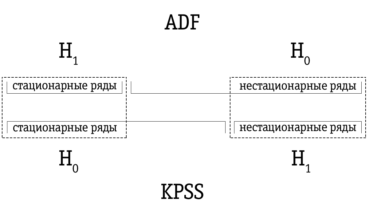
Due to the low power, the Dickey-Fuller test often erroneously identifies a series as non-stationary, so the resulting set of time series identified by the Dickey-Fuller test as unsteady is larger compared to many time series identified as non-stationary using the KPSS test. Therefore, the testing order is important.
If the time series is identified as stationary using the Dickey-Fuller test, then it will most likely also be identified as stationary using the KPSS test; in this case, we can assume that the series is indeed stationary.
If the time series was identified as unsteady using the KPSS test, then it will most likely also be identified as unsteady using the Dickey-Fuller test; in this case, we can assume that the series is indeed unsteady.
However, it often happens that a time series that has been identified as non-stationary using the Dickey-Fuller test will be marked as stationary using the KPSS test. In this case, we must be very careful with our final conclusion. We can check how strong the basis for stationarity is in the case of the KPSS test and for unsteadiness in the case of the Dickey-Fuller test and make an appropriate decision. Of course, we can also leave the question of the stationarity of such a time series unresolved.
KPSS test approach assumes time seriestested for stationarity relative to a trend can be decomposed into the sum of a deterministic trend  random walk
  and stationary error
  :
:
Where - normal iid process with zero mean and variance
  (
( ) Initial value
 treated as fixed and plays the role of a free member. Stationary errorcan be generated by any common ARMA process, that is, it can have strong autocorrelation.
Similar to the Dickey-Fuller test, the ability to take into account an arbitrary structure of autocorrelationvery important because most economic time series are highly time dependent and therefore have a strong autocorrelation. If we want to check the stationarity with respect to the horizontal axis, then the termjust excluded from the equation above.
From the equation above it follows that the null hypothesis about stationarity equivalent to the hypothesis
  , from which it follows that
  for all
  (Is a constant). Similarly, an alternative hypothesis
 non-stationarity is equivalent to the hypothesis
  .
.
To test the hypothesis: (stationary time series) versus alternative : (non-stationary time series) authors of the KPSS test receive one-way statistics of the Lagrange multiplier test. They also calculate its asymptotic distribution and model the asymptotic critical values. We do not consider theoretical details here, but only briefly outline the test execution algorithm.
When performing the KPSS test for a time series,  the least squares method (least squares) is used to estimate one of the following equations:
If we want to check the stationarity with respect to the horizontal axis, we evaluate the first equation. If we plan to check the stationarity with respect to the trend, we choose the second equation.
Leftovers from the estimated equation are used to calculate the statistics of the test of Lagrange multipliers. The Lagrange multiplier test is based on the idea that when the null hypothesis is fulfilled, all the Lagrange multipliers must be equal to zero.
The Lagrange multiplier test is associated with a more general approach to parameter estimation using the maximum likelihood method (ML). According to this approach, data is considered evidence related to distribution parameters. The evidence is expressed as a function of unknown parameters - a likelihood function:
Where Are the observed values, and
  - parameters that we want to evaluate.
The maximum likelihood function is the joint probability of sample observations.
The goal of the maximum likelihood method is to maximize the likelihood function. This is achieved by differentiating the maximum probability function for each of the estimated parameters and equating the partial derivatives to zero. The values of the parameters at which the value of the function is maximum is the desired estimate.
Usually, to simplify the subsequent work, the logarithm of the likelihood function is first taken.
Consider a generalized linear model where it is assumed that
  normally distributed
  , i.e
, i.e  .
.
We want to test the hypothesis that the system (
( ) independent linear constraints
  . Here
 - famous
  rank matrix , a
  - famous
  vector.
For each pair of observed values and under normal conditions, a probability density function of the following form will exist:
On condition joint observations and the total probability of observing all the values in the sample is equal to the product of the individual values of the probability density function. Thus, the likelihood function is defined as follows:
Since it is easier to differentiate the sum than the product, the logarithm of the likelihood function is usually taken, thus:
This useful conversion does not affect the final result, because Is an increasing function
  . So then the value
 which maximizes will also maximize .
ML score for in regression with restriction () is obtained by maximizing the function  on condition . To find this estimate, we write the Lagrange function:
where through marked vector Lagrange multipliers.
Lagrange multiplier test statistics denoted by in case of stationarity with respect to the horizontal axis and through
  in case of stationarity relative to the trend, it is determined by the expression
Where
and
Where
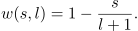
In the above equations - the process of partial balances from the estimated equation;
  - assessment of long-term dispersion of residues ; a
 - the so-called Bartlett spectral window, where
  - lag truncation parameter.
In this application, the spectral window is used to estimate the spectral density of errors for a certain interval (window), which moves along the entire range of the series. Data outside the interval is ignored, since the window function is a function equal to zero outside some selected interval (window).
Variance Estimation depends on the parameter , and since increases and more than 0, score begins to take into account possible autocorrelation in residuals .
Finally, the Lagrange multiplier test statistics or compares with critical values. If the statistics of the Lagrange multiplier test exceeds the corresponding critical value, then the null hypothesis (stationary time series) deviates in favor of an alternative hypothesis (non-stationary time series). Otherwise, we cannot reject the null hypothesisabout stationarity of a time series.
Critical values are asymptotic and, therefore, are most suitable for large sample sizes. However, in practice they are also used for a small sample. Moreover, the critical values are independent of the parameter. However, the statistics of the Lagrange multiplier test will depend on the parameter. The authors of the KPSS test do not offer any general algorithm for choosing the appropriate parameter.. The test is usually performed forin the range from 0 to 8.
When increasing we are less likely to reject the null hypothesis about stationarity, which partially leads to a decrease in the power of the test and can give mixed results. However, in general, we can say that if the null hypothesis stationarity of the time series is not rejected even at small values (0, 1 or 2), we conclude that the verified time series are stationary.
The following methodology was developed to assess the likelihood of symmetry.
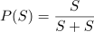
All calculations are performed using the MATLAB package. The results are presented in the table below. For each test, we have a number of relations that are symmetrical according to the test results (marked ); we have a number of relationships that are not symmetrical according to the test results (marked); and we have an empirical probability that the ratio is symmetrical according to the test results (
 )
)
On the Moscow Exchange:
On the New York Stock Exchange:
Let's compare the results of a trading strategy on historical data for co-integrated pairs selected using the Angle-Granger test and for co-integrated pairs selected using the KPSS test.
As can be seen from the table, due to a more accurate identification of co-integrated pairs of shares, it was possible to increase the average annual yield when trading a separate co-integrated pair by 9.21%. Thus, the proposed methodology can increase the profitability of algorithmic trading using market-neutral strategies.
As we saw above, the results of the Angle-Granger test are a lottery. To some, my thoughts will seem overly categorical, but I think it makes great sense not to take the null hypothesis, confirmed by statistical analysis, on faith.
The conservatism of the scientific method for testing hypotheses is that when analyzing the data we can only make one valid conclusion: the null hypothesis is rejected at the chosen level of significance. This does not mean that the alternative is true.- we just received indirect evidence of its credibility on the basis of a typical "evidence from the contrary." In the case when it is true, the researcher is also instructed to make a cautious conclusion: based on the data obtained in the experimental conditions, it was not possible to find enough evidence to reject the null hypothesis.
In unison with my thoughts in September 2018, an article was written by influential people calling to abandon the concept of “statistical significance” and the paradigm of testing the null hypothesis.
Most importantly: “Suggestions such as changing the threshold level -the default values, the use of confidence intervals with an emphasis on whether they contain zero or not, or the use of the Bayes coefficient along with universally accepted classifications to assess the strength of evidence that comes from all the same or similar problems as the current use -values with a level of 0.05 ... are a form of statistical alchemy that makes a false promise to transform randomness into reliability, the so-called “washing of uncertainty” (Gelman, 2016), which begins with data and ends with dichotomous conclusions about truth or falsity - binary statements that “there is an effect” or “no effect” - on the basis of achieving some -values or other threshold value.
A critical step forward will be the acceptance of uncertainty and variability of effects (Carlin, 2016; Gelman, 2016), the recognition that we can learn more (much more) about the world, abandoning the false promise of certainty offered by such dichotomization. ”
We saw that although the symmetry property of the cointegration relation should theoretically be satisfied, the experimental data diverge from theoretical calculations. One of the interpretations of this paradox is the low power of the Dickey-Fuller test.
As a new methodology for identifying co-integrated asset pairs, it was proposed to test the regression residues obtained using the Angle-Granger test for stationarity using the KPSS test and combine the results of these tests; and combine the results of the Angle-Granger test and the KPSS test for both direct and reverse regression.
Backtests were conducted on the data of the Moscow Exchange for 2017. According to the results of backtests, the average annual yield when using the methodology for identifying cointegrated pairs of shares proposed above was 22.72%. Thus, compared with the identification of co-integrated stock pairs using the Angle-Granger test, it was possible to increase the average annual yield by 9.21%.
An alternative interpretation of the paradox is to not take the null hypothesis, confirmed by statistical analysis, on faith. The null hypothesis testing paradigm and the dichotomy offered by such a paradigm give us a false sense of market knowledge.
When I just started my research, it seemed to me that you can take the market, put it into the "meat grinder" of statistical tests and get filtered tasty rows at the exit. Unfortunately, now I see that this concept of statistical brute force will not work.
Whether there is cointegration on the market or not - for me this question remains open. I still have big questions for the founders of this theory. I used to have some trepidation in the West and those scientists who developed financial mathematics at a time when econometrics was considered a corrupt bourgeoisie in the Soviet Union. It seemed to me that we were very far behind, and somewhere in Europe and America the gods of finance were sitting, who knew the sacred grail of truth.
Now I understand that European and American scientists are not much different from ours, the only difference is in the scale of quackery. Our scientists are sitting in an ivory castle, they write some nonsense and receive grants in the amount of 500 thousand rubles. In the West, about the same scientists are sitting in about the same ivory castle, they write about the same nonsense and get "nobel" and grants in the amount of 500 thousand dollars for this. That’s the whole difference.
At the moment, I do not have a clear view of the subject of my research. It is wrong to say that “all hedge funds use pair trading” because most hedge funds go bankrupt just as well.
Unfortunately, you always have to think and make decisions with your own head, especially when we risk money.
co-integrated with nearby , row not always co-integrated with a number . If we study cointegration purely theoretically, then it is easy to prove that if the series
co-integrated with then row co-integrated with . However, if we begin to study cointegration empirically, it turns out that theoretical calculations are not always confirmed. Why it happens?Symmetry
Attitude
called symmetric if where - the inverse ratio defined by the condition: tantamount to . In other words, if the relationthen the relation . Consider two
a number of and , . Cointegration is symmetric if entails that is, if the presence of direct regression leads to the presence of the inverse. Consider the equation
, . Swap the left and right sides and subtract from both parts: . Because by definition, divide both parts into :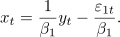
Replace
on the , a on the we get . Therefore, the cointegration relation is symmetric. It follows that if the variable
cointegrated with variable then the variable must be co-integrated with the variable . However, the Angle-Granger cointegration test does not always confirm this symmetry property, since sometimes a variable not co-integrated with variable according to this test. I tested the symmetry property on the 2017 data of the Moscow and New York exchanges using the Angle-Granger test. There were 7,975 co-integrated pairs of shares on the Moscow Exchange. For 7731 (97%) cointegrated pairs, the symmetry property was confirmed, for 244 (3%) cointegrated pairs the symmetry property was not confirmed.
There were 140,903 co-integrated pairs of shares on the New York Stock Exchange. For 136586 (97%) cointegrated pairs, the symmetry property was confirmed, for 4317 (3%) cointegrated pairs the symmetry property was not confirmed.
Interpretation
This result can be interpreted by the low power and high probability of error of the second kind of the Dickey-Fuller test, on which the Angle-Granger test is based. The probability of a second kind error can be denoted by
then the value called the power of the test. Unfortunately, the Dickey-Fuller test is not able to distinguish between non-stationary and near-non-stationary time series. What is a near-unsteady time series? Consider the time series
. A stationary time series is a series in which. A non-stationary time series is a series in which. A near-unsteady time series is a series in which the valueclose to one. In the case of near-non-stationary time series, we are often not able to reject the null hypothesis of non-stationary. This means that the Dickey-Fuller test has a high risk of a second kind error, that is, the probability of not rejecting the false null hypothesis.
KPSS test
A possible response to the weakness of the Dickey-Fuller test is the KPSS test, which owes its name to the initials of the scientists of Kvyatkovsky, Phillips, Schmidt and Sheen. Although the methodological approach of this test is completely different from the Dickey-Fuller approach, the main difference should be understood in the permutation of the null and alternative hypotheses.
In the KPSS test, the null hypothesis states that the time series is stationary, versus the alternative about the presence of non-stationarity. Near-non-stationary time series, which were often identified as non-stationary using the Dickey-Fuller test, can be correctly identified as stationary using the KPSS test.
However, we must be aware that any results of statistical testing are merely probabilistic and should not be confused with a certain true judgment. There is always a non-zero probability that we are mistaken. For this reason, it is proposed to combine the results of the Dickey-Fuller and KPSS tests as an ideal test for non-stationarity.
Due to the low power, the Dickey-Fuller test often erroneously identifies a series as non-stationary, so the resulting set of time series identified by the Dickey-Fuller test as unsteady is larger compared to many time series identified as non-stationary using the KPSS test. Therefore, the testing order is important.
If the time series is identified as stationary using the Dickey-Fuller test, then it will most likely also be identified as stationary using the KPSS test; in this case, we can assume that the series is indeed stationary.
If the time series was identified as unsteady using the KPSS test, then it will most likely also be identified as unsteady using the Dickey-Fuller test; in this case, we can assume that the series is indeed unsteady.
However, it often happens that a time series that has been identified as non-stationary using the Dickey-Fuller test will be marked as stationary using the KPSS test. In this case, we must be very careful with our final conclusion. We can check how strong the basis for stationarity is in the case of the KPSS test and for unsteadiness in the case of the Dickey-Fuller test and make an appropriate decision. Of course, we can also leave the question of the stationarity of such a time series unresolved.
KPSS test approach assumes time series
tested for stationarity relative to a trend can be decomposed into the sum of a deterministic trend random walk and stationary error :
Where
- normal iid process with zero mean and variance () Initial valuetreated as fixed and plays the role of a free member. Stationary errorcan be generated by any common ARMA process, that is, it can have strong autocorrelation. Similar to the Dickey-Fuller test, the ability to take into account an arbitrary structure of autocorrelation
very important because most economic time series are highly time dependent and therefore have a strong autocorrelation. If we want to check the stationarity with respect to the horizontal axis, then the termjust excluded from the equation above. From the equation above it follows that the null hypothesis
about stationarity equivalent to the hypothesis , from which it follows that for all (Is a constant). Similarly, an alternative hypothesis non-stationarity is equivalent to the hypothesis . To test the hypothesis
: (stationary time series) versus alternative : (non-stationary time series) authors of the KPSS test receive one-way statistics of the Lagrange multiplier test. They also calculate its asymptotic distribution and model the asymptotic critical values. We do not consider theoretical details here, but only briefly outline the test execution algorithm. When performing the KPSS test for a time series
, the least squares method (least squares) is used to estimate one of the following equations:
If we want to check the stationarity with respect to the horizontal axis, we evaluate the first equation. If we plan to check the stationarity with respect to the trend, we choose the second equation.
Leftovers
from the estimated equation are used to calculate the statistics of the test of Lagrange multipliers. The Lagrange multiplier test is based on the idea that when the null hypothesis is fulfilled, all the Lagrange multipliers must be equal to zero.Lagrange multiplier test
The Lagrange multiplier test is associated with a more general approach to parameter estimation using the maximum likelihood method (ML). According to this approach, data is considered evidence related to distribution parameters. The evidence is expressed as a function of unknown parameters - a likelihood function:

Where
Are the observed values, and - parameters that we want to evaluate. The maximum likelihood function is the joint probability of sample observations.

The goal of the maximum likelihood method is to maximize the likelihood function. This is achieved by differentiating the maximum probability function for each of the estimated parameters and equating the partial derivatives to zero. The values of the parameters at which the value of the function is maximum is the desired estimate.
Usually, to simplify the subsequent work, the logarithm of the likelihood function is first taken.
Consider a generalized linear model
where it is assumed that normally distributed , i.e . We want to test the hypothesis that the system
() independent linear constraints . Here - famous rank matrix , a - famous vector. For each pair of observed values
and under normal conditions, a probability density function of the following form will exist:
On condition
joint observations and the total probability of observing all the values in the sample is equal to the product of the individual values of the probability density function. Thus, the likelihood function is defined as follows:
Since it is easier to differentiate the sum than the product, the logarithm of the likelihood function is usually taken, thus:

This useful conversion does not affect the final result, because
Is an increasing function . So then the valuewhich maximizes will also maximize . ML score for
in regression with restriction () is obtained by maximizing the function on condition . To find this estimate, we write the Lagrange function:
where through
marked vector Lagrange multipliers. Lagrange multiplier test statistics denoted by
in case of stationarity with respect to the horizontal axis and through in case of stationarity relative to the trend, it is determined by the expression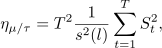
Where

and

Where
In the above equations
- the process of partial balances from the estimated equation; - assessment of long-term dispersion of residues ; a - the so-called Bartlett spectral window, where - lag truncation parameter. In this application, the spectral window is used to estimate the spectral density of errors for a certain interval (window), which moves along the entire range of the series. Data outside the interval is ignored, since the window function is a function equal to zero outside some selected interval (window).
Variance Estimation
depends on the parameter , and since increases and more than 0, score begins to take into account possible autocorrelation in residuals . Finally, the Lagrange multiplier test statistics
or compares with critical values. If the statistics of the Lagrange multiplier test exceeds the corresponding critical value, then the null hypothesis (stationary time series) deviates in favor of an alternative hypothesis (non-stationary time series). Otherwise, we cannot reject the null hypothesisabout stationarity of a time series. Critical values are asymptotic and, therefore, are most suitable for large sample sizes. However, in practice they are also used for a small sample. Moreover, the critical values are independent of the parameter
. However, the statistics of the Lagrange multiplier test will depend on the parameter. The authors of the KPSS test do not offer any general algorithm for choosing the appropriate parameter.. The test is usually performed forin the range from 0 to 8. When increasing
we are less likely to reject the null hypothesis about stationarity, which partially leads to a decrease in the power of the test and can give mixed results. However, in general, we can say that if the null hypothesis stationarity of the time series is not rejected even at small values (0, 1 or 2), we conclude that the verified time series are stationary.Test Results Comparison
The following methodology was developed to assess the likelihood of symmetry.
- All time series are checked for 1st order integrability using the Dickey-Fuller test at a significance level of 0.05. Only integrable series of the first order are considered below.
- Из интегрируемых рядов 1-го порядка, полученных в п. 1, составляются пары путём сочетания без повторений.
- Пары акций, составленные в п. 2, тестируются на коинтеграцию с помощью теста Энгла-Грэнджера. В результате выявляются коинтегрированные пары.
- Остатки от регрессии, полученные в результате тестирования в п. 3, тестируются на стационарность с помощью теста KPSS. Таким образом, результаты двух тестов объединяются.
- Временные ряды в коинтегрированных парах из п. 2 переставляются местами и снова проверяются на коинтеграцию с помощью теста Энгла-Грэнджера, то есть мы исследуем, является ли отношение между временными рядами симметричным.
- The time series in the co-integrated pairs from item 4 are interchanged and the residuals from the regression are checked again for stationarity using the KPSS test, that is, we will examine whether the relationship between the time series is symmetric.
All calculations are performed using the MATLAB package. The results are presented in the table below. For each test, we have a number of relations that are symmetrical according to the test results (marked
); we have a number of relationships that are not symmetrical according to the test results (marked); and we have an empirical probability that the ratio is symmetrical according to the test results () On the Moscow Exchange:
| Test | ADF | ADF + KPSS |
|---|---|---|
| 7731 | 16 |
| 244 | 1 |
 | 97% | 94% |
On the New York Stock Exchange:
| Test | ADF | ADF + KPSS |
|---|---|---|
| 136586 | 182 |
| 4317 | 7 |
| 97% | 96% |
Backtest Results Comparison
Let's compare the results of a trading strategy on historical data for co-integrated pairs selected using the Angle-Granger test and for co-integrated pairs selected using the KPSS test.
| Criteria | ADF | ADF + KPSS |
|---|---|---|
| The number of symmetric pairs | 6417 | 205 |
| Maximum profit | 340.31% | 287.35% |
| Maximum loss | -53.28% | -46.35% |
| Steam traded in plus | 2904 | 113 |
| Steam traded at zero | 293 | 3 |
| Steam traded in minus | 3220 | 89 |
| Average annual return | 13.51% | 22.72% |
As can be seen from the table, due to a more accurate identification of co-integrated pairs of shares, it was possible to increase the average annual yield when trading a separate co-integrated pair by 9.21%. Thus, the proposed methodology can increase the profitability of algorithmic trading using market-neutral strategies.
Alternative interpretation
As we saw above, the results of the Angle-Granger test are a lottery. To some, my thoughts will seem overly categorical, but I think it makes great sense not to take the null hypothesis, confirmed by statistical analysis, on faith.
The conservatism of the scientific method for testing hypotheses is that when analyzing the data we can only make one valid conclusion: the null hypothesis is rejected at the chosen level of significance. This does not mean that the alternative is true.
- we just received indirect evidence of its credibility on the basis of a typical "evidence from the contrary." In the case when it is true, the researcher is also instructed to make a cautious conclusion: based on the data obtained in the experimental conditions, it was not possible to find enough evidence to reject the null hypothesis. In unison with my thoughts in September 2018, an article was written by influential people calling to abandon the concept of “statistical significance” and the paradigm of testing the null hypothesis.
Most importantly: “Suggestions such as changing the threshold level
-the default values, the use of confidence intervals with an emphasis on whether they contain zero or not, or the use of the Bayes coefficient along with universally accepted classifications to assess the strength of evidence that comes from all the same or similar problems as the current use -values with a level of 0.05 ... are a form of statistical alchemy that makes a false promise to transform randomness into reliability, the so-called “washing of uncertainty” (Gelman, 2016), which begins with data and ends with dichotomous conclusions about truth or falsity - binary statements that “there is an effect” or “no effect” - on the basis of achieving some -values or other threshold value. A critical step forward will be the acceptance of uncertainty and variability of effects (Carlin, 2016; Gelman, 2016), the recognition that we can learn more (much more) about the world, abandoning the false promise of certainty offered by such dichotomization. ”
conclusions
We saw that although the symmetry property of the cointegration relation should theoretically be satisfied, the experimental data diverge from theoretical calculations. One of the interpretations of this paradox is the low power of the Dickey-Fuller test.
As a new methodology for identifying co-integrated asset pairs, it was proposed to test the regression residues obtained using the Angle-Granger test for stationarity using the KPSS test and combine the results of these tests; and combine the results of the Angle-Granger test and the KPSS test for both direct and reverse regression.
Backtests were conducted on the data of the Moscow Exchange for 2017. According to the results of backtests, the average annual yield when using the methodology for identifying cointegrated pairs of shares proposed above was 22.72%. Thus, compared with the identification of co-integrated stock pairs using the Angle-Granger test, it was possible to increase the average annual yield by 9.21%.
An alternative interpretation of the paradox is to not take the null hypothesis, confirmed by statistical analysis, on faith. The null hypothesis testing paradigm and the dichotomy offered by such a paradigm give us a false sense of market knowledge.
When I just started my research, it seemed to me that you can take the market, put it into the "meat grinder" of statistical tests and get filtered tasty rows at the exit. Unfortunately, now I see that this concept of statistical brute force will not work.
Whether there is cointegration on the market or not - for me this question remains open. I still have big questions for the founders of this theory. I used to have some trepidation in the West and those scientists who developed financial mathematics at a time when econometrics was considered a corrupt bourgeoisie in the Soviet Union. It seemed to me that we were very far behind, and somewhere in Europe and America the gods of finance were sitting, who knew the sacred grail of truth.
Now I understand that European and American scientists are not much different from ours, the only difference is in the scale of quackery. Our scientists are sitting in an ivory castle, they write some nonsense and receive grants in the amount of 500 thousand rubles. In the West, about the same scientists are sitting in about the same ivory castle, they write about the same nonsense and get "nobel" and grants in the amount of 500 thousand dollars for this. That’s the whole difference.
At the moment, I do not have a clear view of the subject of my research. It is wrong to say that “all hedge funds use pair trading” because most hedge funds go bankrupt just as well.
Unfortunately, you always have to think and make decisions with your own head, especially when we risk money.