Automatic task assignment in Jira using ML
Hello, Habr! My name is Sasha and I am a backend developer. In my free time I study ML and have fun with hh.ru data.
This article is about how we automated the routine task assignment process for testers using machine learning.
Hh.ru has an internal service for which tasks are created in Jira (inside the company they are called HHS) if someone doesn’t work or is working incorrectly. Further, these tasks are manually handled by the QA team leader Alexey and assigned to the team whose area of responsibility includes the malfunction. Lesha knows that boring tasks must be performed by robots. Therefore, he turned to me for help regarding ML.

The graph below shows the amount of HHS per month. We are growing and the number of tasks is growing. Tasks are mainly created during working hours, a few per day, and this has to be constantly distracted.
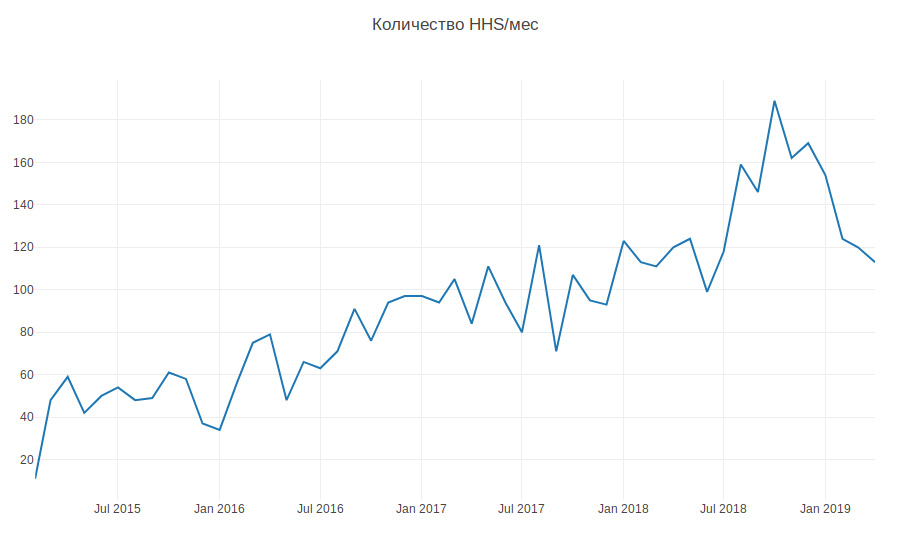
So, according to historical data, it is necessary to learn how to determine the development team to which HHS belongs. This is a multi-class classification task.
In machine learning tasks, the most important thing is quality data. The outcome of the solution to the problem depends on them. Therefore, any machine learning tasks need to start with studying the data. Since the beginning of 2015, we have accumulated about 7000 tasks that contain the following useful information:
Let's start with the target variable. Firstly, each team has areas of responsibility. Sometimes they intersect, sometimes one team may intersect in development with another. The decision will be based on the assumption that the assignee, which remained with the task at the time of closure, is responsible for its solution. But we need to predict not a specific person, but a team. Fortunately, all the teams in Jira are kept and can be mapped. But there are a number of problems with the definition of a team by person:
After filtering out irrelevant data, the training sample was reduced to 4900 tasks.
Let's look at the distribution of tasks between teams:

Tasks need to be distributed between 22 teams.
Summary and Description are text fields.
First, they should be cleaned of excess characters. For some tasks, it makes sense to leave in the lines characters that carry information, for example + and #, to distinguish between c ++ and c #, but in this case I decided to leave only letters and numbers, because did not find where other characters might be useful.
Words need to be lemmatized. Lemmatization is the reduction of a word to a lemma, its normal (vocabulary) form. For example, cats → cat. I also tried stemming, but with lemmatization the quality was a little higher. Stamming is the process of finding the basis of a word. This basis is due to the algorithm (in different implementations they are different), for example, by cats → cats. The meaning of the first and second is to juxtapose the same words in different forms. I used the python wrapper forYandex Mystem .
Further, the text should be cleared of stop words that do not carry a payload. For example, “was”, “me”, “yet”. Stop words I usually take from NLTK .
Another approach that I try in the tasks of working with text is a character-based fragmentation of words. For example, there is a “search”. If you break it into components of 3 characters, you get the words "poi", "ois", "lawsuit". This helps to get additional connections. Suppose there is the word “search”. Lemmatization does not lead to “search” and “search” in a general form, but a partition of 3 characters will highlight the common part - “claim”.
I made two tokens. Tokenizer is a method that receives text at the input, and the list of tokens that make up the text is output. The first highlights lemmatized words and numbers. The second only highlights lemmatized words, which are divided into 3 characters, i.e. at the output, he has a list of three-character tokens.
Tokenizers are used in TfidfVectorizer , which is used to convert text (and not only) data into a vector representation based on tf-idf. A list of rows is fed to it at the input, and at the output we get a matrix M by N, where M is the number of rows and N is the number of signs. Each feature is a frequency response of a word in a document, where the frequency is fined if the word occurs many times in all documents. Thanks to the ngram_range TfidfVectorizer parameter, I added bigrams and trigrams as attributes .
I also tried using word embeddings obtained with Word2vec as additional features. Embedding is a vector representation of a word. For each text, I averaged the embeddings of all his words. But this did not give any increase, so I refused these signs.
For Labels CountVectorizer was used. The rows with tags are fed to the input, and at the output we have a matrix where the rows correspond to the tasks and the columns correspond to the tags. Each cell contains the number of occurrences of the tag in the task. In my case, it is 1 or 0. LabelBinarizer
came up for Reporter . It binarizes one-to-all attributes. There can only be one creator for each task. At the entrance to the LabelBinarizer, a list of task creators is submitted, and the output is a matrix, where the rows are tasks and the columns correspond to the names of the task creators. It turns out that in each line there is “1” in the column corresponding to the creator, and in the rest - “0”. For Created, the difference in days between the date the task was created and the current date is considered. As a result, the following signs were obtained:
All these signs are combined into one large matrix (4855, 129478), on which training will be carried out.
Separately, it is worth noting the names of the signs. Because some machine learning models can identify features that have the greatest impact on class recognition, you need to use this. TfidfVectorizer, CountVectorizer, LabelBinarizer have get_feature_names methods that display a list of features whose order corresponds to columns of data matrices.
Very often XGBoost gives good results . And he began with it. But I generated a huge number of features, the number of which significantly exceeds the size of the training sample. In this case, the probability of retraining XGBoost is high. The result is not very good. High dimension is well digested LogisticRegression . She showed higher quality.
I also tried as an exercise to build a model on a neural network in Tensorflow using this excellent tutorial, but it turned out worse than with a logistic regression.
I also played with the XGBoost and Tensorflow hyperparameters, but I leave it outside the post, because the result of logistic regression was not surpassed. At the last I twisted all the pens that could be. All parameters as a result remained default, except for two: solver = 'liblinear' and C = 3.0
Another parameter that can affect the result is the size of the training sample. Because I am dealing with historical data, and over the course of several years the history can seriously change, for example, responsibility for something can go to another team, then more recent data can be more useful, and old data can even lower quality. In this regard, I came up with heuristics - the older the data, the less contribution they should make to model training. Depending on the age, the data are multiplied by a certain coefficient, which is taken from the function. I generated several functions to attenuate the data and used the one that gave the greatest increase in testing.
Due to this, the quality of classification increased by 3%
In classification problems, we need to think about what is more important for us - accuracy or completeness ? In my case, if the algorithm is wrong, then there is nothing to worry about, we have very good knowledge between the teams and the task will be transferred to those responsible, or to the main one in QA. In addition, the algorithm does not make mistakes randomly, but finds a command close to the problem. Therefore, it was decided to take 100% for completeness. And for measuring quality, the accuracy metric was chosen - the proportion of correct answers, which for the final model was 76%.
As a validation mechanism, I first used cross-validation - when the sample is divided into N parts and quality is checked on one part, and training is carried out on the rest, and so N times, until each part is tested. The result is then averaged. But in my case, this approach did not fit, because the order of the data is changing, and as it has already become known, quality depends on the freshness of the data. Therefore, I studied all the time on old ones, and was validated on fresh ones.
Let's see which teams are most often confused by the algorithm:

In the first place are Marketing and Pandora. This is not surprising since the second team grew out of the first and took away responsibility for many functionalities. If you consider the rest of the team, you can also see the reasons associated with the internal kitchen of the company.
For comparison, I want to look at random models. If you assign a responsible person randomly, then the quality will be about 5%, and if for the most common class, then - 29%
LogisticRegression for each class returns attribute coefficients. The greater the value, the greater the contribution this attribute made to this class.
Under the spoiler, the output of the top of the signs. Prefixes indicate where the signs came from:
Signs roughly reflect what the teams are doing.
On this, the construction of the model is completed and it is possible to build a program on its basis.
The program consists of two Python scripts. The first builds a model, and the second makes predictions.
To make the program convenient to deploy and have the same library versions as during development, scripts are packaged in a Docker container.
As a result, we automated the routine process. The accuracy of 76% is not too big, but in this case the misses are not critical. All tasks find their performers, and most importantly, for this, you no longer need to be distracted several times a day to understand the essence of the tasks and look for those responsible. Everything works automatically! Hurrah!
This article is about how we automated the routine task assignment process for testers using machine learning.
Hh.ru has an internal service for which tasks are created in Jira (inside the company they are called HHS) if someone doesn’t work or is working incorrectly. Further, these tasks are manually handled by the QA team leader Alexey and assigned to the team whose area of responsibility includes the malfunction. Lesha knows that boring tasks must be performed by robots. Therefore, he turned to me for help regarding ML.
The graph below shows the amount of HHS per month. We are growing and the number of tasks is growing. Tasks are mainly created during working hours, a few per day, and this has to be constantly distracted.
So, according to historical data, it is necessary to learn how to determine the development team to which HHS belongs. This is a multi-class classification task.
Data
In machine learning tasks, the most important thing is quality data. The outcome of the solution to the problem depends on them. Therefore, any machine learning tasks need to start with studying the data. Since the beginning of 2015, we have accumulated about 7000 tasks that contain the following useful information:
- Summary - Title, Short Description
- Description - a complete description of the problem
- Labels - a list of tags related to the problem
- Reporter is the name of the creator of HHS. This feature is useful because people work with a limited set of functionalities.
- Created - Creation Date
- Assignee is the person to whom the task is assigned. The target variable will be generated from this attribute.
Let's start with the target variable. Firstly, each team has areas of responsibility. Sometimes they intersect, sometimes one team may intersect in development with another. The decision will be based on the assumption that the assignee, which remained with the task at the time of closure, is responsible for its solution. But we need to predict not a specific person, but a team. Fortunately, all the teams in Jira are kept and can be mapped. But there are a number of problems with the definition of a team by person:
- not all HHS are related to technical problems, and we are only interested in those tasks that can be assigned to the development team. Therefore, you need to throw out tasks where the assignee is not from the technical department
- sometimes teams cease to exist. They are also removed from the training set.
- Unfortunately, people do not work forever in the company, and sometimes they move from team to team. Fortunately, we managed to get a history of the composition of all teams. Having the creation date of HHS and assignee, you can find which team was engaged in the task at a specific time.
After filtering out irrelevant data, the training sample was reduced to 4900 tasks.
Let's look at the distribution of tasks between teams:
Tasks need to be distributed between 22 teams.
Signs:
Summary and Description are text fields.
First, they should be cleaned of excess characters. For some tasks, it makes sense to leave in the lines characters that carry information, for example + and #, to distinguish between c ++ and c #, but in this case I decided to leave only letters and numbers, because did not find where other characters might be useful.
Words need to be lemmatized. Lemmatization is the reduction of a word to a lemma, its normal (vocabulary) form. For example, cats → cat. I also tried stemming, but with lemmatization the quality was a little higher. Stamming is the process of finding the basis of a word. This basis is due to the algorithm (in different implementations they are different), for example, by cats → cats. The meaning of the first and second is to juxtapose the same words in different forms. I used the python wrapper forYandex Mystem .
Further, the text should be cleared of stop words that do not carry a payload. For example, “was”, “me”, “yet”. Stop words I usually take from NLTK .
Another approach that I try in the tasks of working with text is a character-based fragmentation of words. For example, there is a “search”. If you break it into components of 3 characters, you get the words "poi", "ois", "lawsuit". This helps to get additional connections. Suppose there is the word “search”. Lemmatization does not lead to “search” and “search” in a general form, but a partition of 3 characters will highlight the common part - “claim”.
I made two tokens. Tokenizer is a method that receives text at the input, and the list of tokens that make up the text is output. The first highlights lemmatized words and numbers. The second only highlights lemmatized words, which are divided into 3 characters, i.e. at the output, he has a list of three-character tokens.
Tokenizers are used in TfidfVectorizer , which is used to convert text (and not only) data into a vector representation based on tf-idf. A list of rows is fed to it at the input, and at the output we get a matrix M by N, where M is the number of rows and N is the number of signs. Each feature is a frequency response of a word in a document, where the frequency is fined if the word occurs many times in all documents. Thanks to the ngram_range TfidfVectorizer parameter, I added bigrams and trigrams as attributes .
I also tried using word embeddings obtained with Word2vec as additional features. Embedding is a vector representation of a word. For each text, I averaged the embeddings of all his words. But this did not give any increase, so I refused these signs.
For Labels CountVectorizer was used. The rows with tags are fed to the input, and at the output we have a matrix where the rows correspond to the tasks and the columns correspond to the tags. Each cell contains the number of occurrences of the tag in the task. In my case, it is 1 or 0. LabelBinarizer
came up for Reporter . It binarizes one-to-all attributes. There can only be one creator for each task. At the entrance to the LabelBinarizer, a list of task creators is submitted, and the output is a matrix, where the rows are tasks and the columns correspond to the names of the task creators. It turns out that in each line there is “1” in the column corresponding to the creator, and in the rest - “0”. For Created, the difference in days between the date the task was created and the current date is considered. As a result, the following signs were obtained:
- tf-idf for Summary in words and numbers (4855, 4593)
- tf-idf for Summary on three character partitions (4855, 15518)
- tf-idf for Description in words and numbers (4855, 33297)
- tf-idf for Description on three-character partitions (4855, 75359)
- number of entries for Labels (4855, 505)
- binary signs for Reporter (4855, 205)
- task lifetime (4855, 1)
All these signs are combined into one large matrix (4855, 129478), on which training will be carried out.
Separately, it is worth noting the names of the signs. Because some machine learning models can identify features that have the greatest impact on class recognition, you need to use this. TfidfVectorizer, CountVectorizer, LabelBinarizer have get_feature_names methods that display a list of features whose order corresponds to columns of data matrices.
Prediction Model Selection
Very often XGBoost gives good results . And he began with it. But I generated a huge number of features, the number of which significantly exceeds the size of the training sample. In this case, the probability of retraining XGBoost is high. The result is not very good. High dimension is well digested LogisticRegression . She showed higher quality.
I also tried as an exercise to build a model on a neural network in Tensorflow using this excellent tutorial, but it turned out worse than with a logistic regression.
Selection of hyperparameters
I also played with the XGBoost and Tensorflow hyperparameters, but I leave it outside the post, because the result of logistic regression was not surpassed. At the last I twisted all the pens that could be. All parameters as a result remained default, except for two: solver = 'liblinear' and C = 3.0
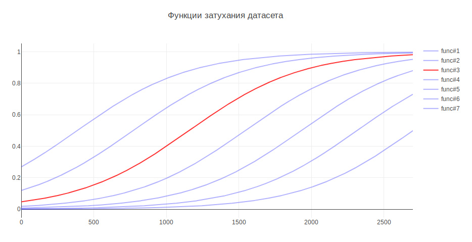
Another parameter that can affect the result is the size of the training sample. Because I am dealing with historical data, and over the course of several years the history can seriously change, for example, responsibility for something can go to another team, then more recent data can be more useful, and old data can even lower quality. In this regard, I came up with heuristics - the older the data, the less contribution they should make to model training. Depending on the age, the data are multiplied by a certain coefficient, which is taken from the function. I generated several functions to attenuate the data and used the one that gave the greatest increase in testing.
Due to this, the quality of classification increased by 3%
Quality control
In classification problems, we need to think about what is more important for us - accuracy or completeness ? In my case, if the algorithm is wrong, then there is nothing to worry about, we have very good knowledge between the teams and the task will be transferred to those responsible, or to the main one in QA. In addition, the algorithm does not make mistakes randomly, but finds a command close to the problem. Therefore, it was decided to take 100% for completeness. And for measuring quality, the accuracy metric was chosen - the proportion of correct answers, which for the final model was 76%.
As a validation mechanism, I first used cross-validation - when the sample is divided into N parts and quality is checked on one part, and training is carried out on the rest, and so N times, until each part is tested. The result is then averaged. But in my case, this approach did not fit, because the order of the data is changing, and as it has already become known, quality depends on the freshness of the data. Therefore, I studied all the time on old ones, and was validated on fresh ones.
Let's see which teams are most often confused by the algorithm:
In the first place are Marketing and Pandora. This is not surprising since the second team grew out of the first and took away responsibility for many functionalities. If you consider the rest of the team, you can also see the reasons associated with the internal kitchen of the company.
For comparison, I want to look at random models. If you assign a responsible person randomly, then the quality will be about 5%, and if for the most common class, then - 29%
The most significant signs
LogisticRegression for each class returns attribute coefficients. The greater the value, the greater the contribution this attribute made to this class.
Under the spoiler, the output of the top of the signs. Prefixes indicate where the signs came from:
- sum - tf-idf for Summary in words and numbers
- sum2 - tf-idf for Summary on three-character splits
- desc - tf-idf for Description in words and numbers
- desc2 - tf-idf for Description on three-character partitions
- lab - Labels field
- rep - field Reporter
Signs
A-Team: sum_site (1.28), lab_responses_and_invitations (1.37), lab_failure_to the employer (1.07), lab_makeup (1.03), sum_work (1.59), lab_hhs (1.19), lab_feedback (1.06), rep_name (1.16), sum_ window (1.13), sum_ break (1.04), rep_name_1 (1.22), lab_responses_seeker (1.0), lab_site (0.92)
API: lab_delete_account (1.12), sum_comment_resume (0.94), rep_name_2 (0.9), rep_name_2 rep_name_4 (0.89), rep_name_5 (0.91), lab_managers_of vacancies (0.87), lab_comments_to_resume (1.85), lab_api (0.86), sum_delete_account (0.86), sum_view (0.91), desc_comment (1.02), rep_name_6 (0.85), rep_name_6 sum_api (1.01)
Android: sum_android (1.77), lab_ios (1.66), sum_application (2.9), sum_hr_mobile (1.4), lab_android (3.55), sum_hr (1.36), lab_mobile_application (3.33), sum_mobile (1.4), rep_name_2 (1.34), sum2_ril (1.27 ), sum_android_application (1.28), sum2_pril_rilo (1.19), sum2_pril_ril (1.27), sum2_ril_loc (1.19), sum2_il_larger (1.19)
Billing: rep_name_7 (3.88), desc_account (3.23), rep_name_8 (3.15), lab_b46_ 4.51), rep_name_10 (2.88), sum_account (3.16), lab_billing (2.41), rep_name_11 (2.27), lab_billing_support (2.36), sum_service (2.33), lab_payment_services (1.92), sum_act (2.26), rep_name_12 (1.92), rep_name_ 2.4)
Brandy: lab_talent assessment (2.17), rep_name_14 (1.87), rep_name_15 (3.36), lab_clickme (1.72), rep_name_16 (1.44), rep_name_17 (1.63), rep_name_18 (1.29), sum_page (1.24), sum_brand (1.39) lab ), sum_constructor (1.59), lab_brand of the page (1.33), sum_description (1.23), sum_description_of the company (1.17), lab_article (1.15)
Clickme: desc_act (0.73), sum_adv_hh (0.65), sum_adv_hh_ru (0.65), sum_hh (0.77) lab_hhs (1.27), lab_bs (1.91), rep_name_19 (1.17), rep_name_20 (1.29), rep_name_21 (1.9), rep_name_8 (1.16), sum_advertising (0.67), sum_placing (0.65), sum_adv (0.65), sum_hh_ua (0.64), sum_click_31 (0.64)
Marketing: lab_region (0.9), lab_brakes_site (1.23), sum_mail (1.32), lab_managers_of vacancies (0.93), sum_calender (0.93), rep_name_22 (1.33), lab_requests (1.25), rep_name_6 (1.53), lab_product_1.55 (reproduction_name_23) ), sum_yandex (1.26), sum_distribution_vacancy (0.85), sum_distribution (0.85), sum_category (0.85), sum_error_function (0.83)
Mercury: lab_services (1.76), sum_captcha (2.02), lab_search_workers (lab, 1.01) 1.68), lab_proforientation (2.53), lab_read_summary (2.21), rep_name_24 (1.77), rep_name_25 (1.56), lab_user_name (1.56), sum_user (1.57), rep_name_26 (1.43), lab_moderation_ vacancy (1.58, rep_name_27 (1.38) 1.36)
Mobile_site: sum_mobile_version (1.32), sum_version_site (1.26), lab_application (1.51), lab_statistics (1.32), sum_mobile_version_site (1.25), lab_mobile_version (5.1), sum_version (1.41), rep_name_28 (1.24), 1 ), lab_jtb (1.07), rep_name_16 (1.12), rep_name_29 (1.05), sum_site (0.95), rep_name_30 (0.92)
TMS: rep_name_31 (1.39), lab_talantix (4.28), rep_name_32 (1.55), rep_name_33 (2.59), sum_вal 0.74), lab_search (0.57), lab_search (0.63), rep_name_34 (0.64), lab_calender (0.56), sum_import (0.66), lab_tms (0.74), sum_hh_ response (0.57), lab_mailing (0.64), sum_talantix (0.6), sum2_ 0.56)
Talantix: sum_system (0.86), rep_name_16 (1.37), sum_talantix (1.16), lab_mail (0.94), lab_xor (0.8), lab_talantix (3.19), rep_name_35 (1.07), rep_name_18 (1.33), lab_personal_data (0.79) ), sum_talantics (0.89), sum_proceed (0.78), lab_mail (0.77), sum_response_stop_view (0.73), rep_name_6 (0.72)
WebServices: sum_vacancy (1.36), desc_pattern (1.32), sum_archive (1.39) phone_name_lab 1.44), rep_name_36 (1.28), lab_lawyers (2.1), lab_invitation (1.27), lab_invitation_for_vacancy (1.26), desc_folder (1.22), lab_selected_results (1.2), lab_key_specifications (1.22), sum_find (1.18), sum_find (1.18), sum 1.17)
iOS: sum_application (1.41), desc_application (1.13), lab_andriod (1.73), rep_name_37 (1.05), lab_mobile_application (1.88), lab_ios (4.55), rep_name_6 (1.41), rep_name_38 (1.35), sum_mobile_application ), sum_mobile (0.98), rep_name_39 (0.74), sum_result_hide (0.88), rep_name_40 (0.81), lab_Duplication of a vacancy (0.76)
Architecture: sum_statistics_response (1.1), rep_name_41 (1.4), lab_views_function (1), workflows (4) 1.0), sum_special offer (1.02), rep_name_42 (1.33), rep_name_24 (1.39), lab_summary (1.52), lab_backoffice (0.99), rep_name_43 (1.09), sum_dependent (0.83), sum_statistics (0.83), lab_replies_worker (0.76), 0.74)
Salary Bank: lab_500 (1.18), lab_authorization (0.79), sum_500 (1.04), rep_name_44 (0.85), sum_500_site (1.03), lab_site (1.54), lab_visibility_name (1.54), lab_price list (1.26), lab_setting_visibility_7 (result) sum_error (0.79), lab_delay_orders (1.33), rep_name_43 (0.74), sum_ie_11 (0.69), sum_500_error (0.66), sum2_say_yite (0.65)
Mobile products: lab_mobile_application (1.69), lab_responses (1.65), sum_applic (1.65), lab_h8lic_ ), lab_employer (0.84), sum_mobile (0.81), rep_name_45 (1.2), desc_d0 (0.87), rep_name_46 (1.37), sum_hr (0.79), sum_incorrect_work_search (0.61), desc_application (0.71), rep_name_47 (0.69), 0.6_name ), sum_work_search (0.59)
Pandora: sum_receive (2.68), desc_receive (1.72), lab_sms (1.59), sum_ letter (2.75), sum_notification_response (1.38), sum_password (1.52), lab_recover_password (1.52), lab_mail_mail summaries (1.91, mail) (1.91) ), lab_mail (1.72), lab_ mail (3.37), desc_ mail (1.69), desc_mail (1.47), rep_name_6 (1.32)
Peppers: lab_save_summary (1.43), sum_resum (2.02), sum_orum (1.57), sum_orum (resume) (1.66) 1.19), lab_summary (1.39), sum_code (1.2), lab_applicant (1.34), sum_index (1.47), sum_index_service (1.47), lab_creating_summary (1.28), rep_name_45 (1.82), sum_greatness (1.47), sum_saving_resumability (1.18) 1.13)
Search-1: sum2_poi_is_search (1.86), sum_loop (3.59), lab_questions_o_search (3.86), sum2_poi (1.86), desc_overs (2.49), lab_observing_summary (2.2), lab_observer (2.32), lab_loop (4.3oopropo_1) (1.62), sum_synonym (1.71), sum_sample (1.62), sum2_isk (1.58), sum2_is_isk (1.57), lab_auto-update_sum (1.57)
Search-2: rep_name_48 (1.13), desc_d1 (1.1), lab_premium_options (1.02, ), sum_search (1.4), desc_d0 (1.2), lab_show_contacts (1.17), rep_name_49 (1.12), lab_13 (1.09), rep_name_50 (1.05), lab_search_of vacancies (1.62), lab_responses_and_invitations (1.61), 1.09_result (lab_1 (response) ), lab_filter_in_responses (1.08)
SuperProducts: lab_contact_information (1.78), desc_address (1.46), rep_name_46 (1.84), sum_address (1.74), lab_selected_resumes (1.45), lab_reviews_worker (1.29), sum_right_shot (1.29), sum_right_range (1.29) ), sum_error_position (1.33), rep_name_42 (1.32), sum_quota (1.14), desc_address_office (1.14), rep_name_51 (1.09)
Signs roughly reflect what the teams are doing.
Model use
On this, the construction of the model is completed and it is possible to build a program on its basis.
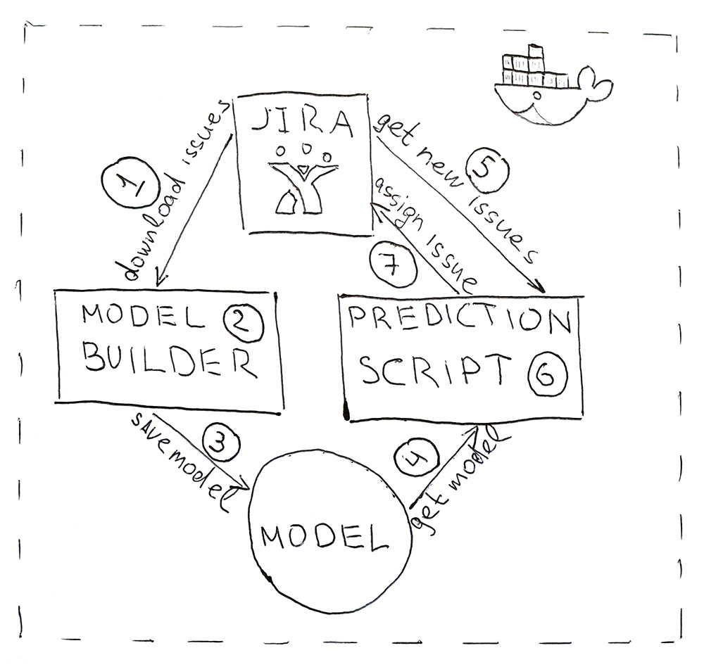
The program consists of two Python scripts. The first builds a model, and the second makes predictions.
- Jira provides an API through which you can download already completed tasks (HHS). Once a day, the script is launched and downloads them.
- Downloaded data is converted to tags. First, the data is beaten for training and test and submitted to the ML-model for validation, to ensure that the quality does not begin to decline from start to start. And then the second time the model is trained on all the data. The whole process takes about 10 minutes.
- The trained model is saved to the hard drive. I used the dill utility to serialize objects. In addition to the model itself, it is also necessary to save all the objects that were used to obtain the characteristics. This is to get signs in the same space for the new HHS.
- Using the same dill, the model is loaded into the script for prediction, which runs once every 5 minutes.
- Go to Jira for the new HHS.
- We get the signs and pass them to the model, which will return for each HHS the class name - the name of the team.
- We find the person responsible for the team and assign him a task through the Jira API. It can be a tester, if the team does not have a tester, then it is a team lead.
To make the program convenient to deploy and have the same library versions as during development, scripts are packaged in a Docker container.
As a result, we automated the routine process. The accuracy of 76% is not too big, but in this case the misses are not critical. All tasks find their performers, and most importantly, for this, you no longer need to be distracted several times a day to understand the essence of the tasks and look for those responsible. Everything works automatically! Hurrah!