An affordable explanation of the Riemann hypothesis
- Transfer
Dedicated to the memory of John Forbes Nash Jr.
Do you remember what "prime numbers" are? These numbers are not divisible by any other than themselves and 1. And now I will ask a question that is already 3000 years old:
- 2, 3, 5, 7, 11, 13, 17, 19, 23, 29, p . What is p equal to ? 31. What will be the next p ? 37. And the next p ? 41. And the next? 43. Yes, but ... how do we know what the next meaning will be?
Come up with a judgment or formula that (at least in sin) predicts what the next prime number (in any given series of numbers) will be, and your name will forever be associated with one of the greatest achievements of the human brain. You will be on a par with Newton, Einstein and Gödel. Understand the behavior of primes, and then you can rest on your laurels all your life.
Introduction
The properties of primes have been studied by many great people in the history of mathematics. From the first proof of the infinity of Euclidean primes to the Euler product formula, which relates primes to the zeta function. From the formulation of the Gauss and Legendre prime theorem to its proof invented by Hadamard and Valle-Poussin. However, Bernhard Riemann is still considered the mathematician who made the single largest discovery in the theory of prime numbers. In his article, published in 1859, consisting of only eight pages, new, previously unknown discoveries were made about the distribution of primes. This article is still considered one of the most important in number theory.
After publication, Riemann's article remained the main work in the theory of primes and in fact became the main reason for proving the theorem on the distribution of primes in 1896 . Since then, several new evidence has been found, including elementary evidence by Selberg and Erdös. However, the Riemann hypothesis about the roots of the zeta function remains a mystery.
How many prime numbers are there?
Let's start with a simple one. We all know that a number is either prime or compound . All compound numbers are simple and can be decomposed into their products (axb). In this sense, prime numbers are the “building blocks” or “fundamental elements” of numbers. In 300 BC, Euclid proved that their number is infinite. His elegant proof is as follows:
Euclidean Theorem
Suppose that the set of primes is not infinite. Create a list of all primes. Then let P be the product of all primes in the list (we multiply all primes from the list). Add to result 1: Q = P +1. Like all numbers, this natural number Q must be either simple or compound:
- If Q is prime, then we have found a prime that is not in our “list of all primes”.
- If Q is not simple, then it is composite, i.e. made up of primes, one of which, p, will be a divisor of Q (because all compound numbers are products of primes). Each prime p from which P is composed is obviously a divisor of P. If p is a divisor for both P and Q, then it must be a divisor for their difference, that is, unity. No prime number is a divisor of 1, so the number p cannot be in the list - another contradiction to the fact that the list contains all primes. There will always be another prime p that is not on the list and is a divisor of Q. Therefore, there are infinitely many primes.
Why are primes so hard to understand?
The fact that any newcomer understands the above problem speaks eloquently about its complexity. Even the arithmetic properties of primes, despite active study, are poorly understood by us. The scientific community is so confident in our inability to understand the behavior of primes that factoring large numbers (defining two primes, the product of which is a number) remains one of the fundamental foundations of encryption theory. You can look at this as follows:
We well understand composite numbers. These are all numbers that are not prime. They consist of primes, but we can easily write a formula that predicts and / or generates composite numbers. Such a "composite number filter" is called a sieve.. The most famous example is the so-called "sieve of Eratosthenes", invented around 200 BC. His job is that it simply marks values that are multiples of each prime number up to a given boundary. Suppose we take the prime number 2 and mark 4,6,8,10, and so on. Then take 3 and mark 6,9,12,15, and so on. As a result, we will only have prime numbers. Although it is very easy to understand, the sieve of Eratosthenes, as you can imagine, is not particularly effective.
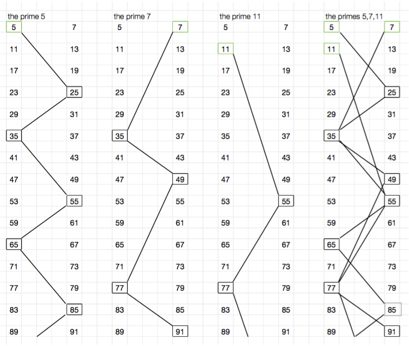
One of the functions that greatly simplifies our work will be 6n ± 1. This simple function returns all primes, with the exception of 2 and 3, and removes all numbers that are multiples of 3, as well as all even numbers. Substitute n = 1,2,3,4,5,6,7 and get the following results: 5,7,11,13,17,19,23,25,29,31,35,37,41,43. The only non-prime numbers generated by the function are 25 and 35, which can be factorized 5 x 5 and 5 x 7. The next non-prime numbers, as you might guess, will be 49 = 7 x 7, 55 = 5 x 11, etc. Everything is easy, right?
To visually display this, I used what I call the “staircase of compound numbers” - a convenient way to show how the composite numbers generated by the function are arranged and combined. In the first three columns of the image below, we see how the prime numbers 5, 7 and 11 climb beautifully up each staircase of composite numbers, up to the value 91. The chaos that occurs in the fourth column, showing how the sieve removed everything except primes, is excellent an illustration of why prime numbers are so hard to understand.
Fundamental resources
How is this all connected with the concept that you could hear about - with the "Riemann hypothesis"? Well, to put it simply, to understand more about primes, mathematicians in the 19th century stopped trying to predict the location of primes with absolute accuracy, and instead began to consider the phenomenon of primes as a whole. Riemann became the master of this analytical approach, and within the framework of this approach his famous hypothesis was created. However, before I begin to explain it, it is necessary to get acquainted with some fundamental resources.
Harmonic Rows
Harmonic series are endless series of numbers that were first explored in the 14th century by Nikolai Orem. His name is associated with the concept of musical harmonics - overtones that are higher than the frequency of the fundamental tone. The rows are as follows:
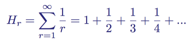
The first members of an infinite harmonic series,
Orem proved that this sum is non-convergent (that is, having no finite limit; it does not approach and does not tend to any particular number, but is directed to infinity).
Zeta functions
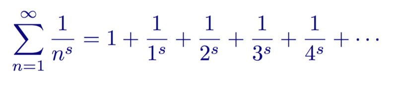
Harmonic series are a special case of a more general type of function called the zeta function ζ (s). The real zeta function is defined for two real numbers r and n :
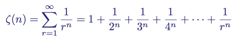
Zeta function
If we substitute n = 1, then we get a harmonic series that diverges. However, for all values of n> 1, the series converges , that is, the sum with increasing r tends to a certain number, and does not go to infinity.
Euler's formula
The first connection between zeta functions and primes was established by Euler when he showed that for two natural (integer and greater than zero) numbers n and p , where p is prime, the following is true:
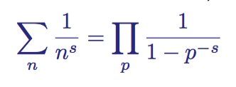
Euler's product for two numbers n and p, where both are greater than zero and p is prime.
This expression first appeared in a 1737 article entitled Variae observationes circa series infinitas . From the expression it follows that the sum of the zeta function is equal to the product of the quantities inverse to unity, minus the inverse of primes of degree s . This stunning connection laid the foundation for the modern theory of primes, in which the zeta function ζ (s) has since begun to be used as a way to study primes.
The proof of the formula is one of my favorite proofs, so I will present it, although for our purposes this is not necessary (but it is just as wonderful!):
Proof of the Euler product formula
Euler starts with a common zeta function
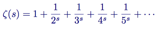
Zeta Function
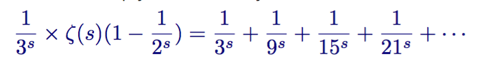
First, he multiplies both parts by the second term:
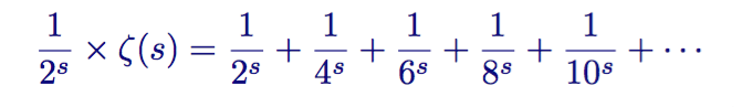
Zeta Function Multiplied by 1/2 s
Then it subtracts the resulting expression from the zeta function:
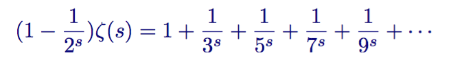
Zeta function minus 1/2 s times the zeta function.
He repeats this process, further multiplying both sides by the third term
Zeta function minus 1/2 s times the zeta function times 1/3 s
And then subtracts the resulting expression from the zeta function
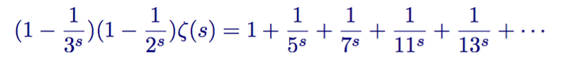
Zeta function minus 1/2 s times the zeta function minus 1/3 s times the zeta function
If you repeat this process indefinitely, in the end we will have the expression:
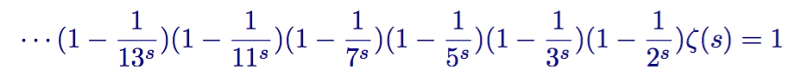
1 minus all the inverse of primes times the zeta function.
If this process is familiar to you, it is because Euler essentially created a sieve very similar to the sieve of Eratosthenes. It filters out non-prime numbers from the zeta function.
Then we divide the expression into all its terms, which are inverse to primes, and get:
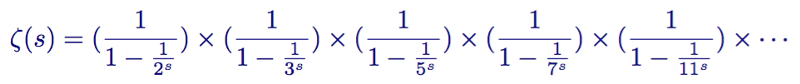
Functional relationship of the zeta function with primes for the first primes 2,3,5,7 and 11 Having simplified the
expression, we showed the following:
The formula for Euler's work is equality, showing the connection between primes and the zeta function.
Wasn't that beautiful? We substitute s = 1, and we find an infinite harmonic series, repeatedly proving the infinity of primes.
Mobius function
August Ferdinand Mobius rewrote the work of Euler, creating a new amount. In addition to the quantities inverse to primes, the Mobius function also contains every natural number, which is the product of an even and odd number of prime factors. Numbers excluded from his series are numbers that are divisible by some prime number squared. Its sum, denoted as μ (n) , has the following form:
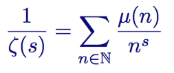
The Mobius function is a modified version of the Euler product given for all natural numbers.
The sum contains the inverse quantities:
- To each prime number;
- To each natural number, which is the product of an odd number of different primes, taken with a minus sign; and
- To each natural number, which is the product of an even number of different primes, taken with a plus sign;
The first members are shown below:
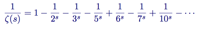
Series / sum of units divided by the zeta function ζ (s)
The sum does not contain those reciprocal quantities that are divided by the square of one of the prime numbers, for example, 4,8,9, and so on.
The Mobius function μ (n) can take only three possible values: the prefix (1 or -1) or the removal (0) of members from the sum:
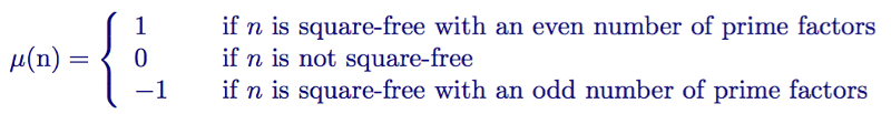
Three possible values of the Mobius function μ (n)
Although this tricky sum was formally determined by Mobius for the first time, it is noteworthy that 30 years before him he wrote about this sum in Gauss margin notes:
“The sum of all primitive roots (prime p) or ≡ 0 (when p-1 is divisible by square), or ≡ ± 1 (mod p) (when p-1 is the product of unequal primes); if their number is even, then the sign is positive, but if the number is odd, then the sign is negative. ”
Prime number distribution function
Let's go back to prime numbers. To understand how primes are distributed when moving up the number line, not knowing exactly where they are, it will be useful to calculate how many of them occur up to a certain number.
It is precisely this task that the distribution function of the primes π (x) proposed by Gauss fulfills: it gives us the number of primes less than or equal to a given real number. Since we do not know the formulas for finding primes, the formula for the distribution of primes is known to us only as a graph, or a step function that increases by 1 when x is a prime. The graph below shows the function up to x = 200.
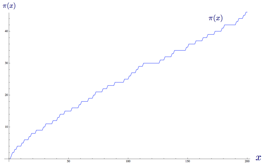
The distribution function of primes π (x) up to x = 200.
Prime number distribution theorem
The theorem on the distribution of primes, formulated by Gauss (and independently Legendre), states:
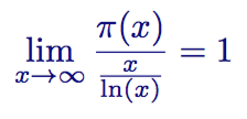
The theorem on the distribution of primes In
ordinary language it can be stated as follows: “When x moves to infinity, the distribution function of the primes π (x) will approach the function x / ln (x)”. In other words, if you climb far enough and the prime distribution graph rises to a very high x , then dividing x by the natural logarithm x, the ratio of these two functions will tend to 1. Below the graph shows two functions for x = 1000:
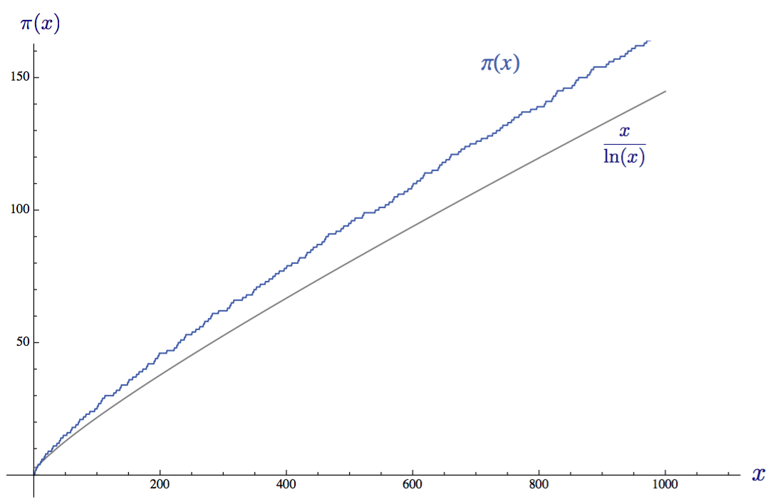
The distribution function of primes π (x) and an approximate estimate by the distribution theorem of primes up to x = 1000
From the point of view of probabilities, the distribution theorem of primes says that if we randomly choose a positive integer x, then the probability P (x) that this number will be prime, approximately equal to 1 / ln (x). This means that the average gap between consecutive primes among the first x integers is approximately ln (x).
Integral Logarithm
The function Li (x) is defined for all positive real numbers, with the exception of x = 1. It is defined by the integral from 2 to x :
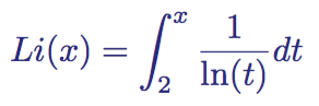
Integral representation of the integral logarithm function
Having built a graph of this function next to the prime distribution function and the formula from the prime distribution theorem, we see that Li (x) is actually a better approximation than x / ln (x):
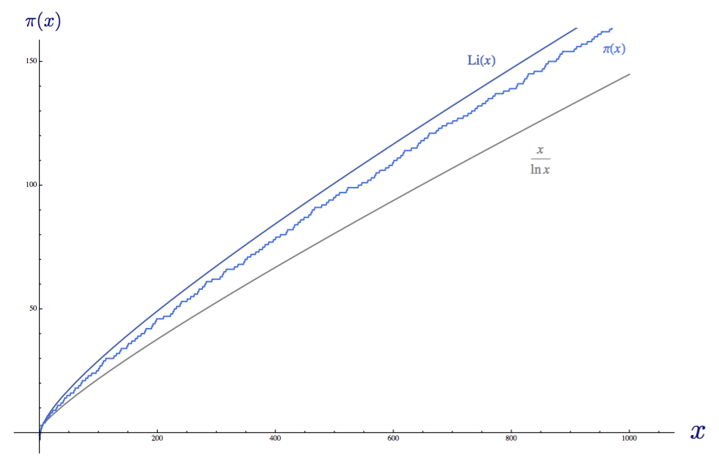
The integral logarithm of Li (x) , the distribution function of primes π (x) and x / ln (x) on one graph.
To find out how much better this approximation is, we can build a table with large x values, the number of primes up to x and the error between the old (theorem on the distribution of primes) and the new (integral logarithm) functions:
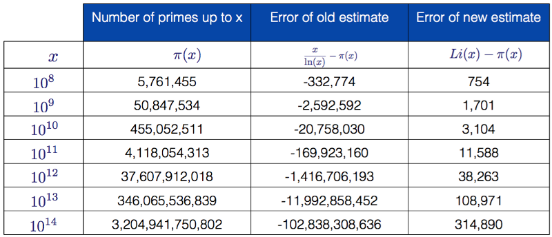
The number of primes to a given power of tens and the corresponding errors for two approximations
As you can easily see, the integral logarithm is much better in the approximation than the function from the theorem on the distribution of primes, it “made a mistake” up to a total of 314,890 primes for x = 10 to the power of 14. Nevertheless, both functions converge to the distribution function of the primes π (x). Li (x) converges much faster, but when x tends to infinity, the ratio between the distribution function of primes and the functions Li (x) and x / ln (x) approaches 1. We show this clearly:
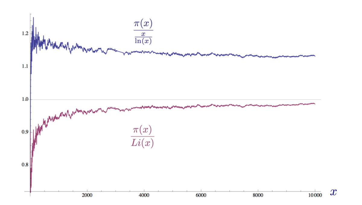
The convergence of the ratios of two approximate values and the distribution function of primes to 1 at x = 10,000
Gamma function
The gamma function Γ (z) has become an important object of study since when in the 1720s, Daniel Bernoulli and Christian Goldbach investigated the problem of generalizing the factorial function to non-integer arguments. This is a generalization of the factorial function n ! (1 x 2 x 3 x 4 x 5 x .... N ) shifted down by 1:
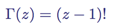
The gamma function defined for z
Her graph is very curious:
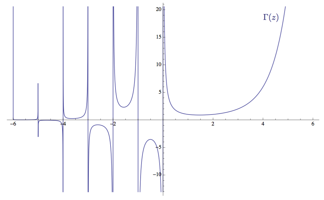
The graph of the gamma function Γ (z) in the interval -6 ≤ z ≤ 6 The
gamma function Γ (z) is defined for all complex values of z greater than zero. As you probably know, complex numbers are a class of numbers with an imaginary part , written as Re ( z ) + Im ( z ), where Re ( z ) is the real part (ordinary real number) and Im ( z ) is the imaginary part denoted by the letter i . The complex number is usually written in the form z = σ + it , where sigma σ is the real part, and it- imaginary. Complex numbers are useful in that they allow mathematicians and engineers to work with problems inaccessible to ordinary real numbers. In complex form, complex numbers extend the traditional one-dimensional number line into a two-dimensional number plane, called the complex plane , in which the real part of the complex number is laid out along the x axis, and the imaginary - along the y axis.
So that the gamma function Γ (z) can be used, it is usually rewritten in the form
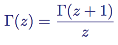
Functional relationship of the gamma function Γ (z)
Using this equality, we can obtain values for z below zero. However, it does not give values for negative integers, because they are not defined (formally they are degenerations or simple poles).
Zeta and gamma
The relationship between the zeta function and the gamma function is given by the following integral:
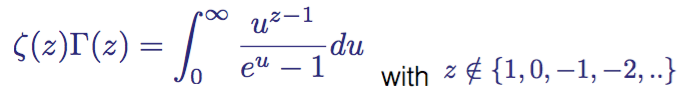
Riemann Zeta Function
Having familiarized ourselves with all the necessary fundamental resources, we can finally begin to establish the connection between the prime numbers and the Riemann hypothesis.
German mathematician Bernhard Riemann was born in 1826 in Brezlenets. As a student of Gauss, Riemann published a paper in the field of mathematical analysis and geometry. It is believed that he made the greatest contribution in the field of differential geometry, where he laid the foundation for the language of geometry, later used by Einstein in the general theory of relativity.
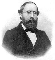
His only work in number theory, an 1859 paper by Ueber die Anzahl der Primzahlen unter einer gegebenen Grösse ("On primes less than a given quantity") is considered the most important article in this area of mathematics. In just four pages he outlined:
- Definition of the Riemann zeta function ζ (s) - zeta function with complex values;
- The analytic continuation of the zeta function to all complex numbers s ≠ 1;
- The definition of the Riemann xi-function ξ (s) - the entire function associated with the Riemann zeta-function through the gamma-function;
- Two proofs of the functional equation of the Riemann zeta function;
- Determination of the distribution function of Riemann primes J (x) using the distribution function of primes and the Mobius function;
- The explicit formula for the number of primes is less than a given number using the distribution function of the Riemann primes defined using the non-trivial zeros of the Riemann zeta function.
This is an incredible example of ingenuity and creative thinking, the likes of which probably have not been seen since. Absolutely amazing work.
Riemann Zeta Function
We have seen the close relationship between primes and the zeta function shown by Euler in his work. However, with the exception of this connection, little was known about their relationship, and the invention of complex numbers was required to show them.
Riemann was the first to consider the zeta function ζ (s) for the complex variable s , where s = σ + i t.
The Riemann zeta function for n, where s = σ + it is a complex number in which σ and t are real numbers.
This infinite series, called the Riemann zeta-function ζ (s), is analytic (that is, has definable values) for all complex numbers with the real part greater than 1 (Re (s)> 1). In this area of definition, it converges absolutely .
To analyze a function in areas outside the usual region of convergence (when the real part of the complex variable s is greater than 1), the function needs to be redefined. Riemann successfully coped with this by performing an analytic continuation to an absolutely convergent function on the half-plane Re (s)> 0.
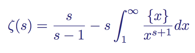
The rewritten form of the Riemann zeta function, where {x} = x - | x |
This new definition of the zeta function is analytic in any part of the half-plane Re (s)> 0, with the exception of s = 1, where it is a degeneracy / simple pole. In this domain of definition, it is called a meromorphic function , because it is holomorphic (complexly differentiable in the neighborhood of each point in the domain of its definition), except for the simple pole s = 1. In addition, it is an excellent example of the Dirichlet L-function .
In his article, Riemann did not stop there. He went over to analytic continuation of his zeta function ζ (s) throughoutcomplex plane using the gamma function Γ (z). In order not to complicate the post, I will not give these calculations, but I highly recommend that you look at them yourself to make sure of the amazing intuition and skill of Riemann.
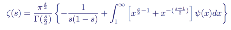
His method uses the integral representation of the gamut Γ (z) for complex variables and the Jacobi theta function ϑ (x), which can be rewritten in such a way that a zeta function appears. When deciding on zeta, we get:
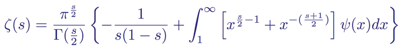
The functional zeta equation for the entire complex plane with the exception of two degeneracies at s = 0 and s = 1
In this form, we notice that the term ψ (s) decreases faster than any power of x, and therefore the integral converges to all values of s.
Going even further, Riemann noticed that the first term in brackets (-1 / s (1 - s)) is an invariant (does not change) if s is replaced by 1 - s. Thanks to this, Riemann further expanded the usefulness of the equation by eliminating two poles at s = 0 and s = 1, and defining the Riemann xi-function ξ (s) without degeneracy:
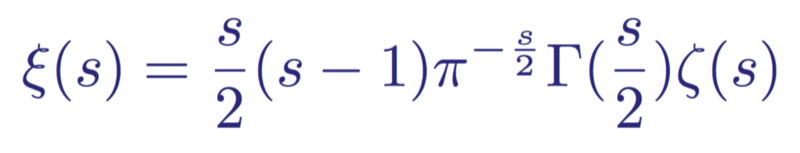
Xi-Riemann function ξ (s)
Zeros of the Riemann Zeta Function
The roots / zeros of the zeta function, when ζ (s) = 0, can be divided into two types, which are called the “trivial” and “nontrivial” zeros of the Riemann zeta function.
The existence of zeros with the real part Re (s) <0
Trivial zeros are zeros that are easy to find and explain. They are most noticeable in the following functional form of the zeta function:
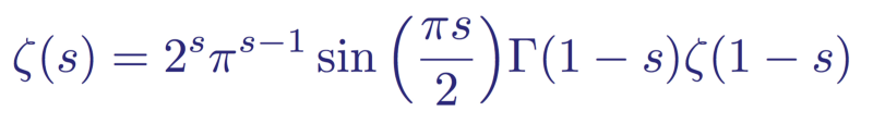
A variation of the Riemann functional zeta equation.
This product becomes equal to zero when the sine becomes zero. This occurs at kπ values. That is, with a negative even integer s = -2n, the zeta function becomes zero. However, for positive even integers s = 2n, the zeros are canceled by the poles of the gamma function Γ (z). It is easier to see in its original functional form; if we substitute s = 2n, then the first part of the term becomes undefined.
So, the Riemann zeta function has zeros in every negative even integer s = -2n. These are trivial zeros, and they can be seen on the function graph:
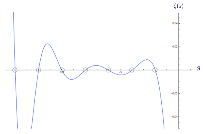
The graph of the Riemann zeta function ζ (s) with zeros at s = -2, -4, -6 and so on
The existence of zeros with the real part Re (s)> 1
From the Euler zeta formulation, we can instantly see that zeta ζ (s) cannot be zero in a region with the real part s greater than 1, because a convergent infinite product can be zero only if one of its factors is equal to zero. The proof of the infinity of primes negates this.
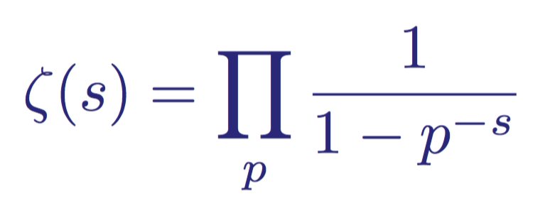
Euler's formula
The existence of zeros with the real part 0 ≤ Re (s) ≤ 1
We found the trivial zeros of the zeta in the negative half-plane when Re (s) <0, and showed that in the region Re (s)> 1 there can be no zeros.
However, the area between these two areas, called the critical strip, has been the main focus of attention in analytic number theory for the past hundreds of years.
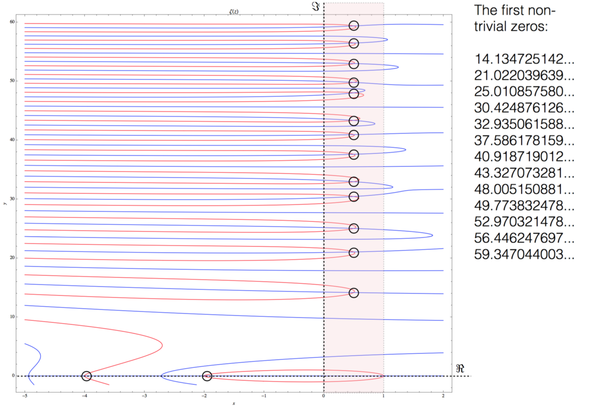
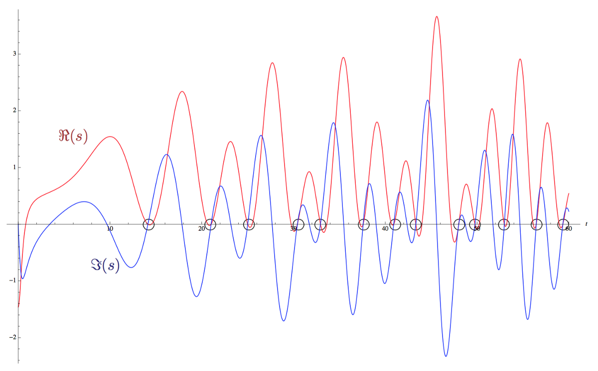
The plot of the real and imaginary parts of the Riemann zeta function ζ (s) in the interval -5 <Re <2, 0 <Im <60
In the graph above, I displayed the real parts of the zeta ζ (s) in red and the imaginary parts in blue. We see the first two trivial zeros in the lower left corner, where the real part of s is -2 and -4. Between 0 and 1, I identified a critical band and noted the intersection of the real and imaginary parts of the zeta ζ (s). These are nontrivial zeros of the Riemann zeta function. Going up to higher values, we will see more zeros and two seemingly random functions that become denser with increasing values of the imaginary part s .
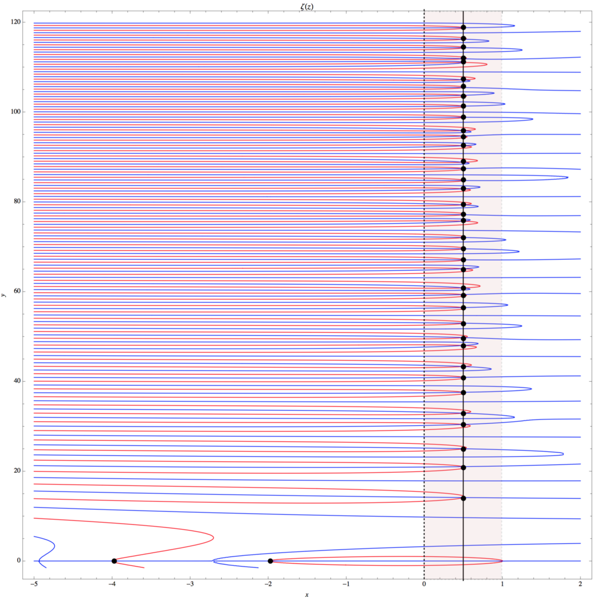
Graph of the real and imaginary parts of the Riemann zeta function ζ (s) in the interval -5 <Re <2, 0 <Im <120
Xi-function Riemann
We defined the Riemann xi-function ξ (s) (the form of a functional equation in which all degeneracy is eliminated, that is, it is defined for all values of s) as follows:
Riemann Xi-function without degeneracy.
This function satisfies the relation
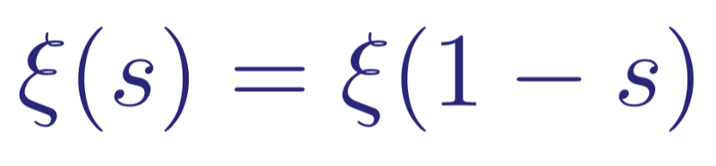
Symmetric relationship between positive and negative values of the Riemann xi-function.
This means that the function is symmetric with respect to the vertical line Re ( s ) = 1/2, i.e. ξ (1) = ξ (0), ξ (2) = ξ (-1 ), etc. This functional connection (symmetries s and 1- s ) in combination with the Euler product shows that the Riemann xi-function can have zeros only in the interval 0 ≤ Re ( s ) ≤ 1. In other words, the zeros of the Riemann xi-functions correspond to non-trivial zeta zeros Riemann functions. In a certain respect, the critical line R (s) = 1/2 for the Riemann zeta function ζ ( s ) corresponds to the real line (Im ( s ) = 0) for the Riemann xi-function ξ ( s ).
Looking at the two graphs shown above, you can immediately notice that for all non-trivial zeros of the Riemann zeta function ζ ( s ) (zeros of the Riemann xi-function), the real part of Re (s) is 1/2. In his article, Riemann briefly mentioned this property, and his superficial note as a result turned out to be one of his greatest legacies.
Riemann hypothesis
For non-trivial zeros of the Riemann zeta-function ζ (s), the real part has the form Re (s) = 1/2.
This is a modern formulation of an unproven assumption made by Riemann in his famous article. It states that all points at which zeta is zero (ζ (s) = 0) on the critical strip 0 ≤ Re (s) ≤ 1 have the real part Re (s) = 1/2. If this is true, then all non-trivial zeros of the zeta will have the form ζ (1/2 + i t).
An equivalent formulation (stated by Riemann himself) is that all the roots of the Riemann xi-function ξ (s) are real.
In the graph below, the line Re (s) = 1/2 is the horizontal axis. The real part Re ( s ) of the zeta ζ ( s ) is shown by the red line, and the imaginary part Im ( s ) is shown by the blue line. Non-trivial zeros are the intersections between the red and blue graphs on the horizontal line.
The first nontrivial zeros of the Riemann zeta function on the line Re (s) = 1/2.
If the Riemann hypothesis turns out to be true, then all non-trivial zeros of the function will occur on this line as the intersection of two graphs.
Reasons to believe in a hypothesis
There are many reasons to believe the truth of the Riemann hypothesis regarding zeros of the zeta function. Probably the most convincing reason for mathematicians is the consequences that it will have for the distribution of primes. A numerical test of a hypothesis at very high values suggests that it is true. In fact, the numerical confirmation of the hypothesis is so strong that in other areas, for example, in physics or chemistry, it could be considered experimentally proven. However, in the history of mathematics there were several hypotheses that were tested to very high values, and nevertheless turned out to be incorrect. Derbyshire (2004) tells the story of the Skews number - an extremely large number that indicated an upper limit and thus proved the falsity of one of the Gauss hypotheses that the integral logarithm of Li ( x) is always greater than the distribution function of primes. It was refuted by Littlewood without an example, and then it was shown that it was incorrect above a very huge number of Skewes - ten to the power of ten, to the power of ten, to the power of 34. This proved that despite the proven fallacy of the Gauss idea, an example of the exact location of such a deviation from the hypothesis is far beyond even modern computing power. This can happen in the case of the Riemann hypothesis, which was tested "only" to tens of twelve non-trivial zeros.
Riemann zeta function and prime numbers
Based on the truth of the Riemann hypothesis, Riemann himself began to study its consequences. In his article, he wrote: "... there is a high probability that all roots are material. Of course, rigorous proof is needed here; after making several unsuccessful attempts, I will postpone its search, because it seems to be optional for the next purpose of my research . " His next goal was to relate zeros of the zeta function to primes.
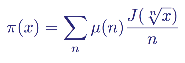
Recall the distribution function of primes π ( x ), which counts the number of primes up to a real number x . Riemann used π ( x ) to determine the eigenfunction of the distribution of primes, namely the distribution function of the Riemann primes J ( x) It is defined as follows:
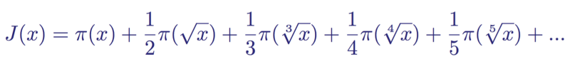
The distribution function of Riemann primes
The first thing that can be noticed in this function is that it is not infinite. For some term, the distribution function will be zero, because there are no primes for x <2. That is, taking J (100) as an example, we get that the function consists of seven members, because the eighth term will contain the eighth root 100, which is approximately equal to 1.778279 .., that is, this term of the distribution of primes becomes equal to zero, and the sum becomes equal to J (100) = 28.5333 ...
Like the distribution function of primes, the Riemann function J ( x ) is a step function, the value which increases like this:
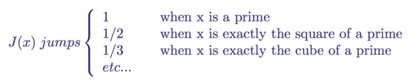
Possible Values of the Riemann Prime Distribution Function
To relate the value of J ( x ) to the number of primes up to x , including it, we will return to the prime distribution function π ( x ) using a process called Mobius inversion (I will not show it here) . The resulting expression will look like
The distribution function of primes π (x) and its connection with the distribution function of Riemann primes and the Mobius function μ (n)
Recall that the possible values of the Mobius function are
Three possible values of the Mobius function μ (n)
This means that now we can write any distribution function of primes as a distribution function of Riemann primes, which will give us

The distribution function of primes, written as the distribution function of Riemann primes for the first seven values of n
This new expression is still a finite sum, because J ( x ) is equal to zero for x <2, since there are no primes less than 2.
If Now we will once again consider the example with J (100), then we get the sum
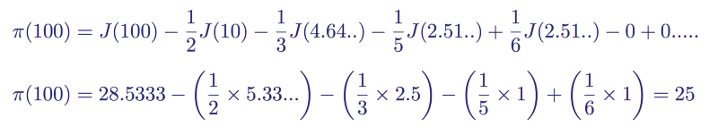
The distribution function of primes for x = 100
Which, as we know, is the number of primes below 100.
Transforming the Euler Product Formula
Then Riemann used Euler's product as a starting point and obtained a method for the analytic estimation of primes in a non-calculable language of matanalysis. Starting with Euler:

Euler's product for the first five primes
First, taking the logarithm on both sides and then rewriting the denominators in brackets, he derived the relationship

Logarithm of the rewritten formula of Euler's product
Then, using the well-known Taylor-Maclaurin series, he expanded each logarithmic term on the right side, creating an infinite sum of infinite sums, one for each term in a series of primes.
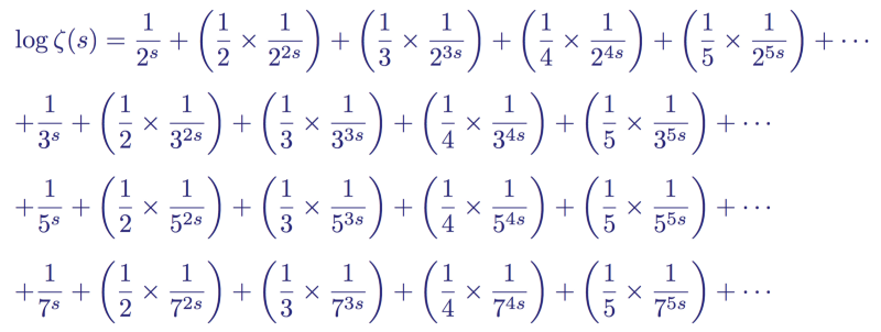
Taylor expansion for the first four members of the logarithm of the Euler product.
Consider one of these members, for example:
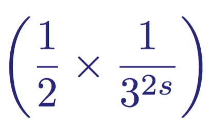
The second term is the Maclaurin expansion for 1/3 ^ s.
This term, like every other calculation term, represents a part of the area under the function J ( x ). In the form of an integral:

The integral form of the second term of the Maclaurin expansion for 1/3 ^ s
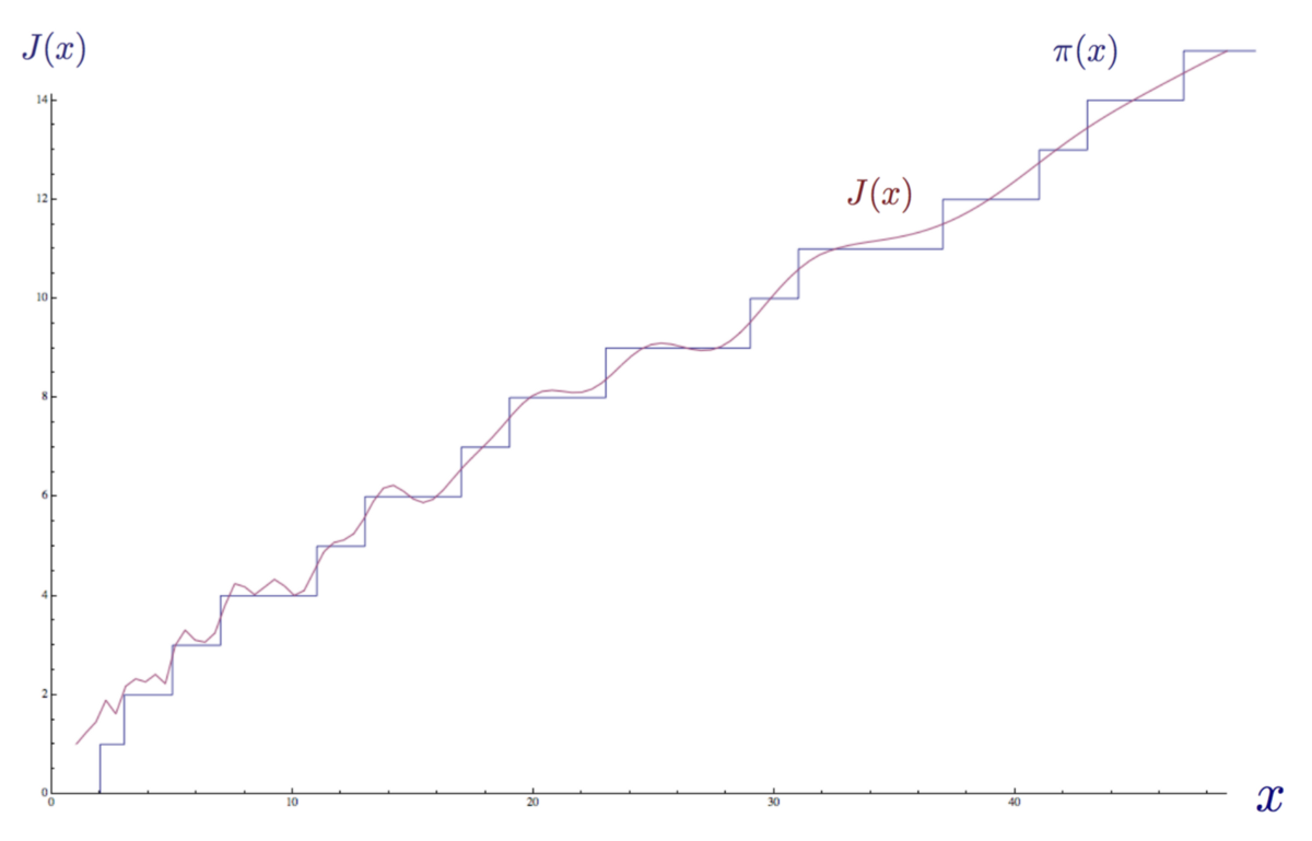
In other words, using the Euler product, Riemann showed that it is possible to represent the discrete stepwise distribution function of primes as a continuous sum of integrals. In the graph below, the example of the term we took is shown as part of the area under the graph of the distribution function of the Riemann primes.
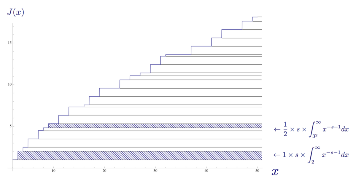
The distribution function of the Riemann primes J (x) up to x = 50, in which two integrals are distinguished.
So, each expression in a finite sum, making up a series of quantities inverse to the primes from the Euler product, can be expressed as integrals making up an infinite sum of integrals, corresponding area under the distribution function of Riemann primes. For a prime number 3, this infinite product of integrals has the form:

An infinite product of the integrals that make up the area under the distribution function of primes represented by an integer 3
If we collect all these infinite sums together into one integral, then the integral under the distribution function of Riemann primes J ( x ) can be written in simple form:
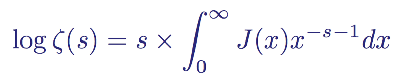
The logarithm of zeta, expressed as an infinite series of integrals
Or in a better known form

The modern equivalent of the Euler product, linking the zeta function with the distribution function of Riemann primes
Thanks to this, Riemann was able to connect in the language of matanalysis his zeta function ζ ( s ) with the distribution function of Riemann primes J ( x ) in an equality equivalent to the formula of the Euler product.
Error
Having obtained this analytical form of the Euler product, Riemann set about formulating his own theorem on the distribution of primes. He presented it in the following explicit form:
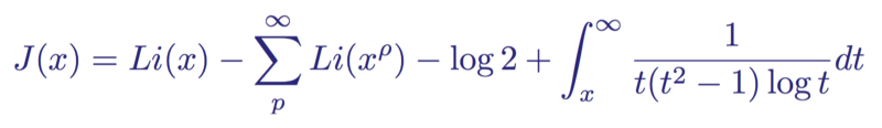
“The Riemann primer distribution theorem,” which predicts the number of primes less than a given quantity x
This is an explicit Riemann formula. It became an improvement of the theorem on the distribution of primes, a more accurate estimate of the number of primes up to the number x . The formula consists of four members:
- Первый, или «основной» член — это интегральный логарифм Li(x), который является улучшенным приближением функции распределения простых чисел π(x) из теоремы о распределении простых чисел. Это самый большой член, и как мы видели, он завышает количество простых чисел до заданного значения x.
- Второй, или «периодический» член — это сумма интегрального логарифма x в степени ρ, суммированная по ρ, что является нетривиальными нулями дзета-функции Римана. Этот член регулирует завышение значений основного члена.
- Третий член — это константа -log(2) = -0.6993147…
- The fourth and last term is the integral, equal to zero for x <2, because there are no primes less than 2. Its maximum value is 2, when its integral is approximately 0.1400101 ....
The influence of the last two terms on the value of the function with increasing x becomes extremely small. The main “contribution” for large numbers is made by the integral logarithm function and the periodic sum. See their effect on the chart:
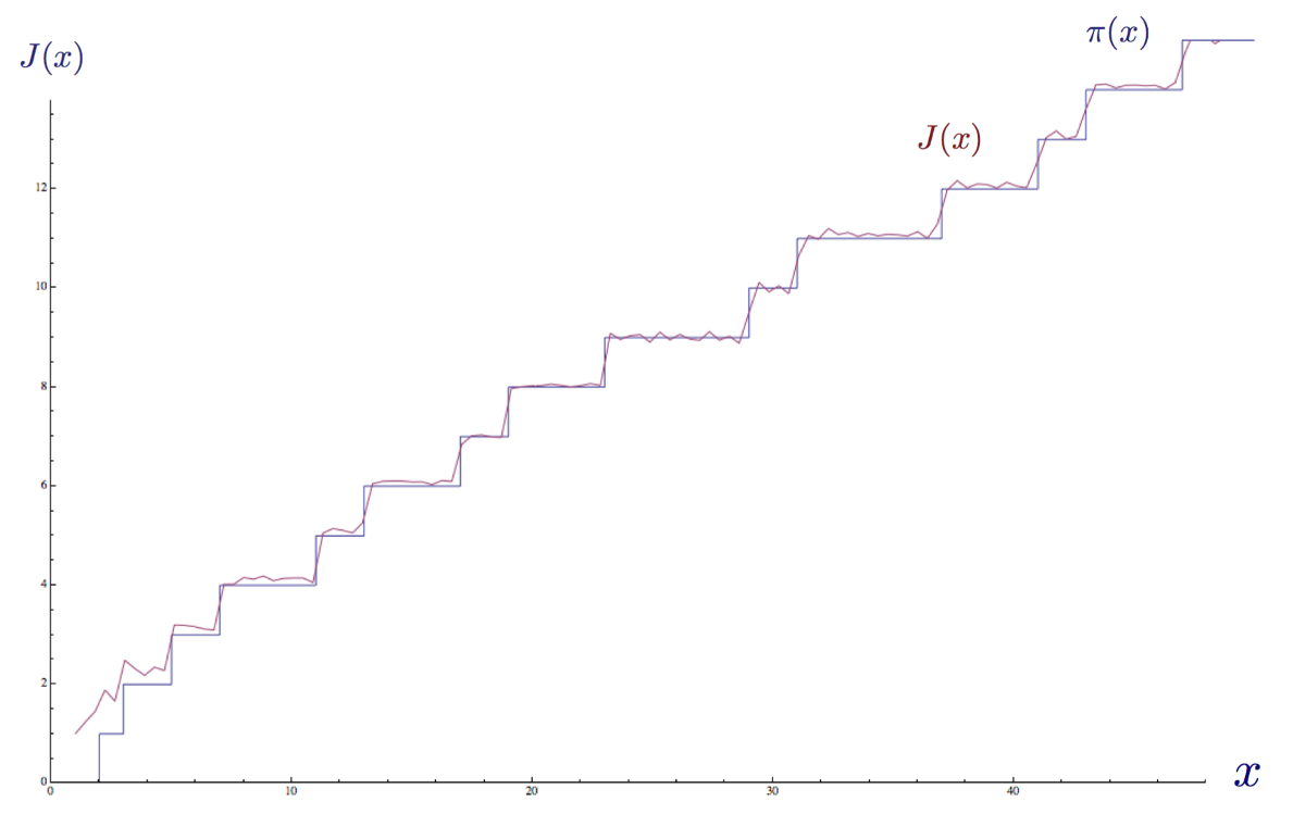
The step function of the distribution of primes π (x) , approximated by the explicit formula for the distribution function of the Riemann primes J (x) using the first 35 nontrivial zeros of the ρ Riemann zeta-function.
In the graph above, I approximated the prime distribution function π ( x ) using the explicit formula of the Riemann prime distribution function J ( x ) and summed the first 35 nontrivial zeros of the Riemann zeta function ζ (s). We see that the periodic term makes the function “resonate” and begin to approach the shape of the distribution function of primes π ( x ).
Below is the same plot using more non-trivial zeros.
The step function of the distribution of primes π (x) approximated by the explicit formula for the distribution of Riemann primes J (x) using the first 100 nontrivial zeros of the ρ Riemann zeta-function.
Using the explicit Riemann function, we can very accurately approximate the number of primes up to a given number x . In fact, in 1901, Niels Koch proved that using non-trivial zeros of the Riemann zeta function to correct the error of the integral logarithm function is equivalent to the “best” boundary for the error in the prime number distribution theorem.
"... These zeros act like telegraph poles, and the special nature of the Riemann zeta function exactly orders how the wire (its graph) should hang between them ...", - Dan Rockmore
Epilogue
After the death of Riemann in 1866, only at the age of 39, his pioneering article continues to be a guide in the field of analytic number theory and the theory of prime numbers. To this day, the Riemann hypothesis of non-trivial zeros of the Riemann zeta function remains unresolved, despite active research by many great mathematicians. Each year, various new results and conjectures are published related to this hypothesis in the hope that someday the evidence will become real.