Short review of the article "DeViSE: A Deep Visual-Semantic Embedding Model"

The article in question.

Introduction

Modern recognition systems are limited to classify into a relatively small number of semantically unrelated classes. Attraction of textual information, even unrelated to the pictures, allows to enrich the model and to some extent solve the following problems:

1. if the recognition model makes an error, then often this error is semantically not close to the correct class;
2. there is no way to predict an object that belongs to a new class that was not represented in the training dataset.

The proposed approach suggests displaying images in a rich semantic space in which labels of more similar classes are closer to each other than labels of less similar classes. As a result, the model gives less semantically distant from the true class of predictions. Moreover, the model, taking into account both visual and semantic proximity, can correctly classify images related to a class that was not represented in the training data set.

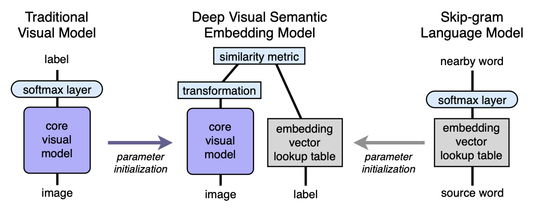
Algorithm. Architecture

1. We pre-train the language model, which gives good semantically meaningful embeddings. The dimension of space is n. Next, n will be taken equal to 500 or 1000.
2. We pre-train the visual model, which classifies objects well into 1000 classes.

3. We cut off the last softmax layer from the pre-trained visual model and add a fully connected layer from 4096 to n neurons. We train the resulting model for each image to predict the embedding corresponding to the image label.

Let us explain with the help of mappings. Let LM be a language model, VM be a visual model with cut off softmax and a fully connected layer added, I - image, L - label of image, LM (L) - label embedding in semantic space. Then in the third step we train the VM so that:

Architecture:

Language model

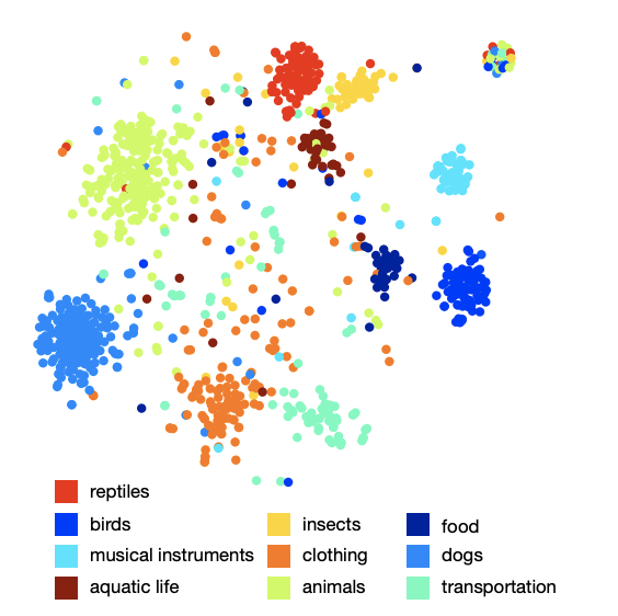
To learn the language model, the skip-gram model was used, a corpus of 5.4 billion words taken from wikipedia.org. The model used a hierarchical softmax layer to predict related concepts, a window - 20 words, the number of passes through the body - 1. It was experimentally established that the embedding size is better to take 500-1000.

The picture of the arrangement of classes in space shows that the model has learned a qualitative and rich semantic structure. For example, for a certain species of sharks in the resulting semantic space, 9 nearest neighbors are the other 9 types of sharks.

Visual model

The architecture that won the 2012 ILSVRC competition was taken as a visual model. Softmax was removed in it and a fully connected layer was added to obtain the desired embedding size at the output.

Loss function

It turned out that the choice of the loss function is important. A combination of cosine similarity and hinge rank loss was used. The loss function encouraged a larger scalar product between the vector of the result of the visual network and the corresponding label labeling and fined for a large scalar product between the result of the visual network and the labelings of random possible image labels. The number of arbitrary random labels was not fixed, but was limited by the condition under which, the sum of scalar products with false labels became more than a scalar product with a valid label minus a fixed margin (constant equal to 0.1). Of course, all vectors were pre-normalized.

Training process

At the beginning, only the last added fully connected layer was trained, the rest of the network did not update the weight. In this case, the SGD optimization method was used. Then the entire visual network was thawed and trained using the Adagrad optimizer so that during back propagation on different layers of the network the gradients scale correctly.

Prediction

During the prediction, from the image using the visual network, we get some vector in our semantic space. Next, we find the nearest neighbors, that is, some possible labels and in a special way display them back in ImageNet synsets for scoring. The procedure for the last display is not so simple, since the labels in ImageNet are a set of synonyms, not just one label. If the reader is interested in knowing the details, I recommend the original article (appendix 2).

results

The result of the DEVISE model was compared with two models:

1. Softmax baseline model - a state-of-the-art vision model (SOTA - at the time of publication)
2. Random embedding model is a version of the described DEVISE model, where embeddings are not learned by the language model, but are initialized arbitrarily.

To assess the quality, “flat” hit @ k metrics and hierarchical precision @ k metric were used. The metric “flat” hit @ k is the percentage of test images for which the correct label is present among the first k predicted options. The hierarchical precision @ k metric was used to evaluate the quality of semantic correspondence. This metric was based on the label hierarchy in ImageNet. For each true label and fixed k, a set of
semantically correct labels was determined - ground truth list. Getting the prediction (nearest neighbors) was the percentage of intersection with the ground truth list.

The authors expected that the softmax model should show the best results on flat metric due to the fact that it minimizes cross-entropy loss, which is very suitable for “flat” hit @ k metrics. The authors were surprised how close the DEVISE model is to the softmax model, reaches parity at large k and even overtakes at k = 20.

On the hierarchical metric, the DEVISE model shows itself in all its glory and overtakes the softmax baseball by 3% for k = 5 and by 7% for k = 20.

Zero-shot learning

A particular advantage of the DEVISE model is the ability to provide adequate prediction for images whose labels the network has never seen during training. For example, during training, the network saw images tagged tiger shark, bull shark, and blue shark and never met the shark mark. Since the language model has a representation for shark in semantic space and is close to embeddings of different types of shark, the model is very likely to give an adequate prediction. This is called the ability to generalize - generalization.

Let's demonstrate some examples of Zero-Shot predictions:

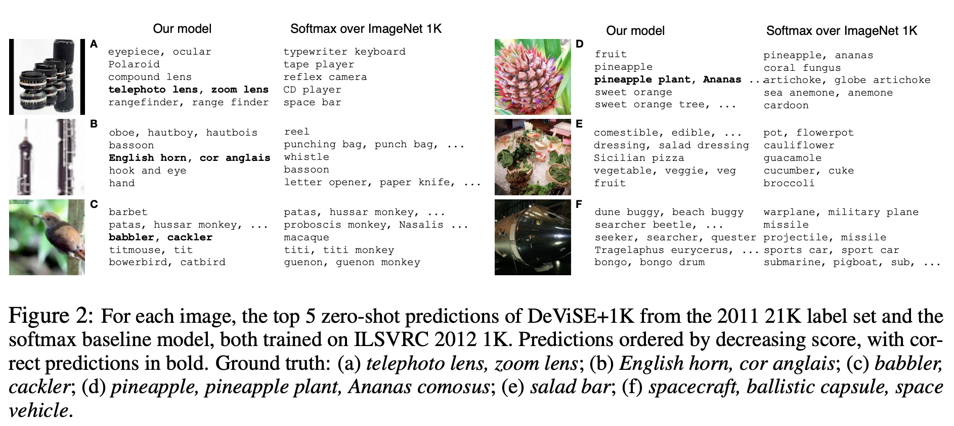
Note that the DEVISE model, even in its erroneous assumptions, is closer to the correct answer than the erroneous assumptions of the softmax model.

So, the presented model loses a bit to softmax to the baseline on flat metrics, but significantly wins on hierarchical precision @ k metric. The model has the ability to generalize, producing adequate predictions for images whose labels the network has not met (zero-shot learning).

The described approach can be easily implemented, as it is based on two pre-trained models - language and visual.