Wavelet Analysis Part 1
- Tutorial
Introduction
Consider the discrete wavelet transform (DWT) implemented in the PyWavelets PyWavelets 1.0.3 library . PyWavelets is a free, open source software released under the MIT license.
When processing data on a computer, a discretized version of the continuous wavelet transform can be performed, the basics of which are described in my previous article . However, specifying discrete values of the parameters (a, b) of wavelets with an arbitrary step Δa and Δb requires a large number of calculations.
In addition, the result is an excessive number of coefficients, far exceeding the number of samples of the original signal, which is not required for its reconstruction.
The discrete wavelet transform (DWT) implemented in the PyWavelets library provides enough information both for signal analysis and for its synthesis, while being economical in terms of the number of operations and the required memory.
When to use the wavelet transform instead of the Fourier transform
The Fourier transform will work very well when the frequency spectrum is stationary. In this case, the frequencies present in the signal are independent of time, and the signal contains the frequencies xHz that are present anywhere in the signal. The unsteady the signal, the worse the results. This is a problem, since most of the signals that we see in real life are unsteady in nature.
The Fourier transform has high resolution in the frequency domain, but zero resolution in the time domain. We show this in the following two examples.
Listing
import numpy as np
from scipy import fftpack
from pylab import*
N=100000
dt = 1e-5
xa = np.linspace(0, 1, num=N)
xb = np.linspace(0, 1/4, num=N/4)
frequencies = [4, 30, 60, 90]
y1a, y1b = np.sin(2*np.pi*frequencies[0]*xa), np.sin(2*np.pi*frequencies[0]*xb)
y2a, y2b = np.sin(2*np.pi*frequencies[1]*xa), np.sin(2*np.pi*frequencies[1]*xb)
y3a, y3b = np.sin(2*np.pi*frequencies[2]*xa), np.sin(2*np.pi*frequencies[2]*xb)
y4a, y4b = np.sin(2*np.pi*frequencies[3]*xa), np.sin(2*np.pi*frequencies[3]*xb)
def spectrum_wavelet(y):
    Fs = 1 / dt  # sampling rate, Fs = 0,1 MHz
    n = len(y)  # length of the signal
    k = np.arange(n)
    T = n / Fs
    frq = k / T  # two sides frequency range
    frq = frq[range(n // 2)]  # one side frequency range
    Y = fftpack.fft(y) / n  # fft computing and normalization
    Y = Y[range(n // 2)] / max(Y[range(n // 2)])
    # plotting the data
    subplot(2, 1, 1)
    plot(k/N , y, 'b')
    ylabel('Amplitude')
    grid()
    # plotting the spectrum
    subplot(2, 1, 2)
    plot(frq[0:140], abs(Y[0:140]), 'r')
    xlabel('Freq')
    plt.ylabel('|Y(freq)|')
    grid()
y= y1a + y2a + y3a + y4a
spectrum_wavelet(y)
show()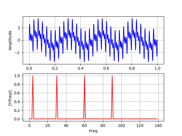
On this graph, all four frequencies are present in the signal during the entire time of its operation.
Listing
import numpy as np
from scipy import fftpack
from pylab import*
N=100000
dt = 1e-5
xa = np.linspace(0, 1, num=N)
xb = np.linspace(0, 1/4, num=N/4)
frequencies = [4, 30, 60, 90]
y1a, y1b = np.sin(2*np.pi*frequencies[0]*xa), np.sin(2*np.pi*frequencies[0]*xb)
y2a, y2b = np.sin(2*np.pi*frequencies[1]*xa), np.sin(2*np.pi*frequencies[1]*xb)
y3a, y3b = np.sin(2*np.pi*frequencies[2]*xa), np.sin(2*np.pi*frequencies[2]*xb)
y4a, y4b = np.sin(2*np.pi*frequencies[3]*xa), np.sin(2*np.pi*frequencies[3]*xb)
def spectrum_wavelet(y):
    Fs = 1 / dt  # sampling rate, Fs = 0,1 MHz
    n = len(y)  # length of the signal
    k = np.arange(n)
    T = n / Fs
    frq = k / T  # two sides frequency range
    frq = frq[range(n // 2)]  # one side frequency range
    Y = fftpack.fft(y) / n  # fft computing and normalization
    Y = Y[range(n // 2)] / max(Y[range(n // 2)])
    # plotting the data
    subplot(2, 1, 1)
    plot(k/N , y, 'b')
    ylabel('Amplitude')
    grid()
    # plotting the spectrum
    subplot(2, 1, 2)
    plot(frq[0:140], abs(Y[0:140]), 'r')
    xlabel('Freq')
    plt.ylabel('|Y(freq)|')
    grid()
y = np.concatenate([y1b, y2b, y3b, y4b])
spectrum_wavelet(y)
show()
On this graph, the signals do not overlap in time, the side lobes are due to a gap between four different frequencies.
For two frequency spectra containing exactly the same four peaks, the Fourier transform cannot determine where these frequencies are present in the signal. The best approach for analyzing signals with a dynamic frequency spectrum is wavelet transform.
The main properties of wavelets
The choice of the type, and therefore the properties of the wavelet, depends on the task of analysis, for example, to determine the effective values of currents in the electric power industry, the higher order waveforms of Ingrid Daubechies provide greater accuracy. Wavelet properties can be obtained using the pywt.DiscreteContinuousWavelet () function in the following listing:
Listing
import pywt
from pylab import *
from numpy import *
discrete_wavelets = ['db5', 'sym5', 'coif5', 'haar']
print('discrete_wavelets-%s'%discrete_wavelets )
st='db20'
wavelet = pywt.DiscreteContinuousWavelet(st)
print(wavelet)
i=1
phi, psi, x = wavelet.wavefun(level=i)
subplot(2, 1, 1)
title("График самой вейвлет - функции -%s"%st)
plot(x,psi,linewidth=2, label='level=%s'%i)
grid()
legend(loc='best')
subplot(2, 1, 2)
title("График первообразной -функции -%s"%st)
plt.plot(x,phi,linewidth=2, label='level=%s'%i)
legend(loc='best')
grid()
show()
Get:
discrete_wavelets - ['db5', 'sym5', 'coif5', 'haar']
Wavelet db20
  Family name:    Daubechies
  Short name:     db
  Filters length: 40
  Orthogonal:     True
  Biorthogonal:   True
  Symmetry:       asymmetric
  DWT:            True
  CWT:            False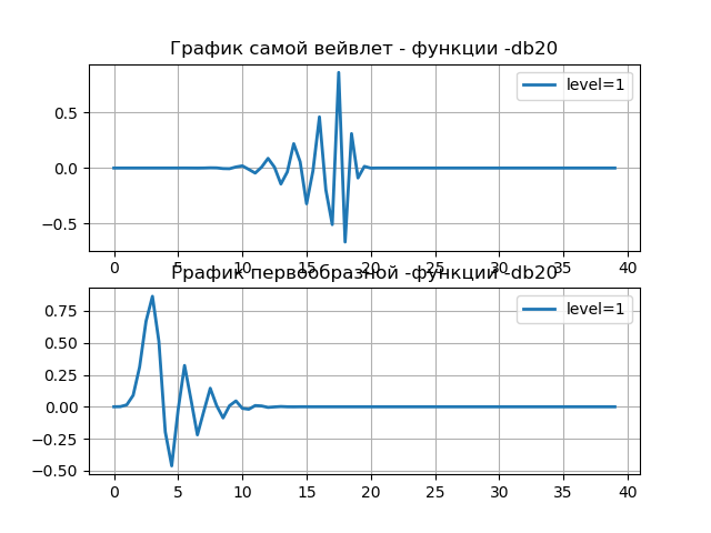
In a number of practical cases, there is a need to obtain information about the central frequency of the psi wavelet - a function that is used, for example, in wavelet analysis of signals to detect defects in gears:
import pywt
fс=pywt.central_frequency('haar', precision=8 )
print(fс)
# или так:
scale=1
fс1=pywt.scale2frequency('haar',scale)
print(fс1)
0.9961089494163424
0.9961089494163424Using the center frequency
 maternal wavelet and scale factor “a” can convert scales to pseudo frequencies
  using the equation:
Signal Extension Modes
Before calculating the discrete wavelet transform using filter banks , it becomes necessary to lengthen the signal . Depending on the extrapolation method, significant artifacts may occur at the signal boundaries, leading to inaccuracies in the DWT transform.
PyWavelets provides several signal extrapolation techniques that can be used to minimize this negative effect. To demonstrate such methods, use the following listing:
Listing demonstration of signal extension methods
import numpy as np
from matplotlib import pyplot as plt
from pywt._doc_utils import boundary_mode_subplot
# synthetic test signal
x = 5 - np.linspace(-1.9, 1.1, 9)**2
# Create a figure with one subplots per boundary mode
fig, axes = plt.subplots(3, 3, figsize=(10, 6))
plt.subplots_adjust(hspace=0.5)
axes = axes.ravel()
boundary_mode_subplot(x, 'symmetric', axes[0], symw=False)
boundary_mode_subplot(x, 'reflect', axes[1], symw=True)
boundary_mode_subplot(x, 'periodic', axes[2], symw=False)
boundary_mode_subplot(x, 'antisymmetric', axes[3], symw=False)
boundary_mode_subplot(x, 'antireflect', axes[4], symw=True)
boundary_mode_subplot(x, 'periodization', axes[5], symw=False)
boundary_mode_subplot(x, 'smooth', axes[6], symw=False)
boundary_mode_subplot(x, 'constant', axes[7], symw=False)
boundary_mode_subplot(x, 'zeros', axes[8], symw=False)
plt.show()
The graphs show how a short signal (red) expands (black) beyond its original length.
Discrete Wavelet Transform
To demonstrate DWT, we will use a signal with a dynamic frequency spectrum, which increases with time. The beginning of the signal contains low-frequency values, and the end of the signal contains frequencies of the short-wave range. This allows us to easily determine which part of the frequency spectrum is filtered out by simply looking at the time axis:
Listing
from pylab import *
from numpy import*
x = linspace(0, 1, num=2048)
chirp_signal = sin(250 * pi * x**2)
fig, ax = subplots(figsize=(6,1))
ax.set_title("Сигнал с динамическим частотным спектром ")
ax.plot(chirp_signal)
show()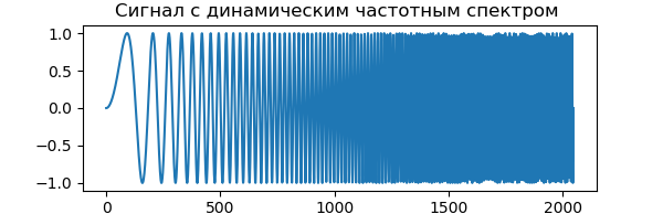
The discrete wavelet transform in PyWavelets 1.0.3 is the pywt.dwt () function, which calculates the approximating coefficients cA and the detailed coefficients cD of the first level wavelet transform of the signal specified by the vector:
Transformation Level One Listing
import pywt
from pylab import *
from numpy import *
x = linspace (0,  1,  num = 2048)
y = sin (250  *  pi * x**2)
st='sym5'
(cA, cD) = pywt.dwt(y,st)
subplot(2, 1, 1)
plot(cA,'b',linewidth=2, label='cA,level-1')
grid()
legend(loc='best')
subplot(2, 1, 2)
plot(cD,'r',linewidth=2, label='cD,level-1')
grid()
legend(loc='best')
show()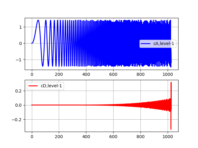
Transformation Level 5 Listing
import pywt
from pylab import *
from numpy import *
x = linspace (0,  1,  num = 2048)
y = sin (250  *  pi * x**2)
st='sym5'
(cA, cD) = pywt.dwt(y,st)
(cA, cD) = pywt.dwt(cA,st)
(cA, cD) = pywt.dwt(cA,st)
(cA, cD) = pywt.dwt(cA,st)
(cA, cD) = pywt.dwt(cA,st)
subplot(2, 1, 1)
plot(cA,'b',linewidth=2, label='cA,level-5')
grid()
legend(loc='best')
subplot(2, 1, 2)
plot(cD,'r',linewidth=2, label='cD,level-5')
grid()
legend(loc='best')
show()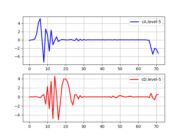
The approximation coefficients (cA) represent the output of the low-pass filter (averaging filter) DWT. The detail coefficients (cD) represent the output of the high-pass filter (differential filter) DWT.
You can use the pywt.wavedec () function to immediately calculate higher-level coefficients. This function takes the input signal and level as input and returns one set of approximation coefficients (n-th level) and n sets of detail coefficients (from 1 to n-th level). Here is an example for the fifth level:
from pywt import wavedec
from pylab import *
from numpy import *
x = linspace (0,  1,  num = 2048)
y = sin (250  *  pi * x**2)
st='sym5'
coeffs = wavedec(y, st, level=5)
subplot(2, 1, 1)
plot(coeffs[0],'b',linewidth=2, label='cA,level-5')
grid()
legend(loc='best')
subplot(2, 1, 2)
plot(coeffs[1],'r',linewidth=2, label='cD,level-5')
grid()
legend(loc='best')
show()
As a result, we get the same graphs as in the previous example. The coefficients cA and cD can be obtained separately:
For cA:
import pywt
from pylab import *
from numpy import*
x = linspace (0,  1,  num = 2048)
data = sin (250  *  pi * x**2)
coefs=pywt.downcoef('a', data, 'db20', mode='symmetric', level=1)
For cD:
import pywt
from pylab import *
from numpy import*
x = linspace (0,  1,  num = 2048)
data = sin (250  *  pi * x**2)
coefs=pywt.downcoef('d', data, 'db20', mode='symmetric', level=1)
Filter bank
Some of the issues related to conversion levels were discussed in the previous section. However, DWT is always implemented as a filter bank in the form of a cascade of high-pass and low-pass filters. Filter banks are a very effective way of dividing a signal into multiple frequency subbands.
At the first stage with a small scale, analyzing the high-frequency behavior of the signal. At the second stage, the scale increases with a factor of two (the frequency decreases with a factor of two), and we analyze the behavior of about half the maximum frequency. At the third stage, the scale factor is four, and we analyze the frequency behavior of about a quarter of the maximum frequency. And this continues until we reach the maximum level of decomposition.
The maximum level of decomposition can be calculated using the pywt.wavedec () function, while decomposition and detail will look like:
Listing
import pywt
from pywt import wavedec
from pylab import *
from numpy import*
x = linspace (0,  1,  num = 2048)
data= sin (250  *  pi * x**2)
n_level=pywt.dwt_max_level(len(data), 'sym5')
print('Максимальный уровень декомпозиции: %s'%n_level)
x = linspace (0,  1,  num = 2048)
y = sin (250  *  pi * x**2)
st='sym5'
coeffs = wavedec(y, st, level=7)
subplot(2, 1, 1)
plot(coeffs[0],'b',linewidth=2, label='cA,level-7')
grid()
legend(loc='best')
subplot(2, 1, 2)
plot(coeffs[1],'r',linewidth=2, label='cD,level-7')
grid()
legend(loc='best')
show()
We get: The
maximum level of decomposition: 7
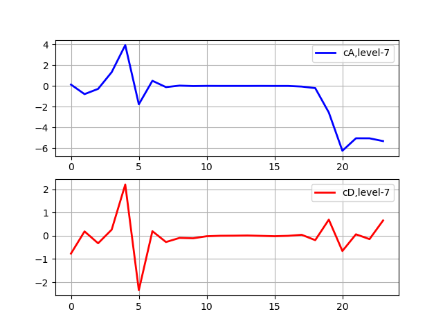
Decomposition stops when the signal becomes shorter than the filter length for this sym5 wavelet. For example, suppose we have a signal with frequencies up to 1000 Hz. At the first stage, we separate our signal into low-frequency and high-frequency parts, i.e. 0-500 Hz and 500-1000 Hz. At the second stage, we take the low-frequency part and again divide it into two parts: 0-250 Hz and 250-500 Hz. In the third stage, we divided the part 0-250 Hz into the part 0-125 Hz and the part 125-250 Hz. This continues until we reach the maximum level of decomposition.
Analysis of wav files using fft Fourier and wavelet scalograms
For analysis, use the WebSDR file . Consider the analysis of the reduced signal using triang from scipy.signal and the implementation of the discrete Fourier transform in python (fft from scipy.fftpack). If the length of the sequence fft is not equal to 2n, then instead of the fast Fourier transform (fft), a discrete Fourier transform (dft) will be performed. This is how this team works.
We use the fast Fourier transform buffer according to the following scheme (numerical data for an example):
fftbuffer = np.zeros (15); create a buffer filled with zeros;
fftbuffer [: 8] = x [7:]; move the end of the signal to the first part of the buffer; fftbuffer [8:] = x [: 7] —we move the beginning of the signal to the last part of the buffer; X = fft (fftbuffer) - we consider the Fourier transform of a buffer filled with signal values.
To make the phase spectrum more readable, phase deployment is applicable. To do this, change the line with the calculation of the phase characteristic: pX = np.unwrap (np.angle (X)).
Listing for fft signal fragment analysis
import numpy as np
from pylab import *
from scipy import *
import scipy.io.wavfile as wavfile
M=501
hM1=int(np.floor((1+M)/2))
hM2=int(np.floor(M/2))
(fs,x)=wavfile.read('WebSDR.wav')
x1=x[5000:5000+M]*np.hamming(M)
N=511
fftbuffer=np.zeros([N])
fftbuffer[:hM1]=x1[hM2:]
fftbuffer[N-hM2:]=x1[:hM2]
X=fft(fftbuffer)
mX=abs(X)
pX=np.angle(X)
suptitle("Анализ радиосигналаWebSDR")
subplot(3, 1, 1)
st='Входной сигнал (WebSDR.wav)'
plot(x,linewidth=2, label=st)
legend(loc='center')
subplot(3, 1, 2)
st=' Частотный спектр входного сигнала'
plot(mX,linewidth=2, label=st)
legend(loc='best')
subplot(3, 1, 3)
st=' Фазовый спектр входного сигнала'
pX=np.unwrap(np.angle(X))
plot(pX,linewidth=2, label=st)
legend(loc='best')
show()
For comparative analysis, we will use a wavelet scalogram that can be built using the tree = pywt.wavedec (signal, 'coif5') function in matplotlib.
Listing Wavelet Scalograms
from pylab import *
import pywt
import scipy.io.wavfile as wavfile
# Найти наибольшую мощность двух каналов, которая меньше или равна входу.
def lepow2(x):
    return int(2 ** floor(log2(x)))
#Скалограмма с учетом дерева MRA.
def scalogram(data):
    bottom = 0
    vmin = min(map(lambda x: min(abs(x)), data))
    vmax = max(map(lambda x: max(abs(x)), data))
    gca().set_autoscale_on(False)
    for row in range(0, len(data)):
        scale = 2.0 ** (row - len(data))
        imshow(
            array([abs(data[row])]),
            interpolation = 'nearest',
            vmin = vmin,
            vmax = vmax,
            extent = [0, 1, bottom, bottom + scale])
        bottom += scale
# Загрузите сигнал, возьмите первый канал.
rate, signal = wavfile.read('WebSDR.wav')
signal = signal[0:lepow2(len(signal))]
tree = pywt.wavedec(signal, 'coif5')
gray()
scalogram(tree)
show()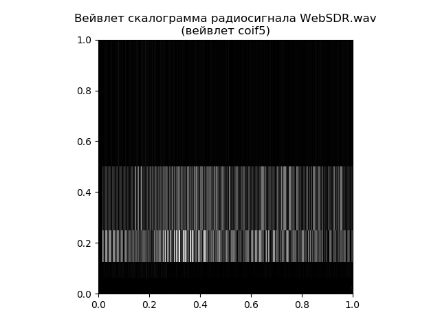
Thus, the scalogram gives a more detailed answer to the question of the distribution of frequencies over time, and the fast Fourier transform is responsible for the frequencies themselves. It all depends on the task, even for such a simple example.
conclusions
- The rationale for using a discrete wavelet transform for dynamic signals is given.
- Examples of wavelet analysis using PyWavelets 1.0.3, a free open source software released under the MIT license, are provided.
- Software tools for practical use of PyWavelets library are considered.