Operating Systems: Three Easy Pieces. Part 5: Planning: Multi-Level Feedback Queue (translation)
Introduction to Operating Systems
Hello, Habr! I want to bring to your attention a series of articles-translations of one interesting literature in my opinion - OSTEP. This article discusses rather deeply the work of unix-like operating systems, namely, work with processes, various schedulers, memory, and other similar components that make up the modern OS. The original of all materials you can see here . Please note that the translation was done unprofessionally (quite freely), but I hope I retained the general meaning.
Laboratory work on this subject can be found here:
Other parts:
- Part 1: Intro
- Part 2: Abstraction: the process
- Part 3: Introduction to the Process API
- Part 4: Introduction to the Scheduler
- Part 5: MLFQ Scheduler
And you can look at my channel in telegram =)
Planning: Multi-Level Feedback Queue
In this lecture, we will talk about the problems of developing one of the most famous
planning approaches , called Multi-Level Feedback Queue (MLFQ). The MLFQ scheduler was first described in 1962 by Fernando J. Corbató in a system called the Compatible Time-Sharing System (CTSS). These works (including later work on Multics) were subsequently submitted to the Turing Award. The scheduler was subsequently improved and acquired a look that can already be found in some modern systems.
The MLFQ algorithm attempts to solve 2 fundamental cross-cutting problems.
At first, he is trying to optimize the turnaround time, which, as we examined in the previous lecture, is optimized by starting at the beginning of the shortest task queue. However, the OS does not know how long this or that process will work, and this is the necessary knowledge for the operation of the SJF, STCF algorithms. SecondlyMLFQ tries to make the system responsive to users (for example, those who sit and stare at the screen while waiting for the task to complete) and thus minimize response time. Unfortunately, algorithms like RR reduce response time, but they have a very bad effect on turnaround time metrics. Hence our problem: How to design a scheduler that will meet our requirements and at the same time know nothing about the nature of the process, in general? How can the scheduler learn the characteristics of the tasks that he launches and thus make better planning decisions?
The essence of the problem: How to plan the formulation of tasks without perfect knowledge? How to develop a scheduler that simultaneously minimizes response time for interactive tasks and at the same time minimizes turnaround time without knowing the time to complete the task?
Note: learning from previous events
The MLFQ line is a great example of a system that learns from past events to predict the future. Similar approaches are often found in the OS (and many other branches in computer science, including hardware prediction branches and caching algorithms). Similar trips work when tasks have behavioral phases and are thus predictable.
However, one should be careful with such a technique, because predictions can very easily turn out to be wrong and lead the system to make worse decisions than would be without knowledge at all.
MLFQ: Basic Rules
Consider the basic rules of the MLFQ algorithm. Although there are several implementations of this algorithm, the basic approaches are similar.
In the implementation that we will consider, in MLFQ there will be several separate queues, each of which will have a different priority. At any time, a task ready for execution is in one queue. MLFQ uses priorities to decide which task to run, i.e. a task with a higher priority (a task from the queue with a higher priority) will be launched first.
Undoubtedly, more than one task can be in a particular queue, so they will have the same priority. In this case, the RR engine will be used to schedule the launch among these tasks.
Thus we come to two basic rules for MLFQ:
- Rule1: If priority (A)> Priority (B), task A will start (B will not)
- Rule2: If priority (A) = Priority (B), A&B are started using RR
Based on the above, the key elements to MLFQ planning are priorities. Instead of setting a fixed priority for each task, MLFQ changes its priority depending on the observed behavior.
For example, if a task constantly quits work on the CPU while waiting for keyboard input, MLFQ will maintain the priority of the process at a high level, because this is how the interactive process should work. If, on the contrary, the task constantly and intensively uses the CPU for a long period, MLFQ will lower its priority. Thus, MLFQ will study the behavior of processes at the time of their operation and use the behavior.
Let's draw an example of how the queues might look at some point in time and then we get something like this:

In this scheme, 2 processes A and B are in the queue with the highest priority. Process C is somewhere in the middle, and process D is at the very end of the queue. According to the above descriptions of the MLFQ algorithm, the scheduler will execute tasks only with the highest priority according to RR, and tasks C, D will be out of work.
Naturally, a static snapshot will not give a complete picture of how MLFQ works.
It is important to understand exactly how the picture changes over time.
Attempt 1: How to change the priority
At this point, you need to decide how MLFQ will change the priority level of the task (and thus the position of the task in the queue) during its life cycle. To do this, you need to keep in mind the workflow: a number of interactive tasks with a short run time (and thus frequent CPU release) and several long tasks that use the CPU all their working time, while the response time for such tasks is not important. And thus, you can make the first attempt to implement the MLFQ algorithm with the following rules:
- Rule3: When a task enters the system, it is queued with the highest
- priority.
- Rule4a: If a task uses the entire time window allotted to it, then its
- priority goes down.
- Rule4b: If the Task frees the CPU before the expiration of its time window, then it
- remains with the same priority.
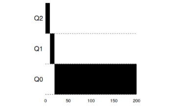
Example 1: A single, long-running task
As you can see in this example, the task is set with the highest priority upon admission. After a time window of 10ms the process is lowered in priority by the scheduler. After the next time window, the task finally drops to the lowest priority in the system, where it remains.
Example 2: We brought up a short task
Now let's see an example of how MLFQ will try to approach SJF. There are two tasks in this example: A, which is a long-running task that constantly takes up the CPU, and B, which is a short interactive task. Suppose A already worked for some time by the time task B arrives.
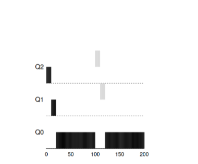
In this graph, the results of the script are visible. Task A, like any task that uses a CPU, is at the very bottom. Task B will arrive at T = 100 and will be placed in the queue with the highest priority. Since the time of her work is short, it will end before it reaches the last stage.
From this example, one should understand the main goal of the algorithm: since the algorithm does not know a long task or a short one, it first of all assumes that the task is short and gives it the highest priority. If this is a really short task, then it will be completed quickly, otherwise if it is a long task, it will slowly move downward in priority and will soon prove that it is a really long task that does not require a response.
Example 3: What about I / O?
Now take a look at the I / O example. As stated in rule 4b, if a process frees a processor without fully utilizing its processor time, then it remains at the same priority level. The intent of this rule is quite simple - if an interactive task performs many I / O operations, for example, waiting for a user to press a key or a mouse, such a task will free the processor before the allotted window. We would not want to omit such a task by priority, and thus it will remain at the same level.

This example shows how the algorithm will work with such processes - an interactive task B, which needs a CPU for only 1ms before performing the I / O process, and a long task A, which uses the CPU all its time.
MLFQ holds process B with the highest priority as it continues to
free up the CPU all the time . If B is an interactive task, then the algorithm then achieved its goal of launching interactive tasks quickly.
Problems with the current MLFQ algorithm
In the previous examples, we built the basic version of MLFQ. And it seems that he does his job well and honestly, distributing processor time honestly between long tasks and allowing short tasks or tasks intensively accessing I / O to work out quickly. Unfortunately, this approach contains several serious problems.
At first, the problem of hunger: if there are a lot of interactive tasks in the system, then they will consume all the processor time and thus not a single long task will get the opportunity to be executed (they are starving).
Secondly , smart users could write their programs in such a way as to
deceive the scheduler. The deception lies in doing something to make the
scheduler give the process more processor time. The algorithm
described above is quite vulnerable to such attacks: before the time window is almost
over, you need to perform an I / O operation (to some file, no matter which file)
and thus free the CPU. This behavior will allow you to stay in the same
the queue itself and again get a larger percentage of CPU time. If you do
it right (for example, 99% of the window's time before the CPU is freed up),
such a task can simply monopolize the processor.
Finally, a program can change its behavior over time. Those tasks
that used the CPU can become interactive. In our example, such
tasks will not receive proper treatment from the scheduler, since they would receive other
(initial) interactive tasks.
Question to the audience: what attacks on the planner could be made in the modern world?
Attempt 2: Raising Priority
Let's try to change the rules and see if we can avoid problems with
starvation. What could we do to ensure that
CPU- related tasks get their time (even if not for long).
As a simple solution to the problem, you can suggest periodically
increasing the priority of all such tasks in the system. There are many ways to
achieve this, let’s try to implement something simple as an example: to transfer
all tasks at once to the highest priority, hence the new rule:
- Rule5 : After a certain period of S, transfer all the tasks in the system to the highest priority.
Our new rule solves two problems at once. Firstly, processes are
guaranteed not to starve: tasks in the highest priority will share
processor time according to the RR algorithm and thus all processes will receive
processor time. Secondly, if some process that previously used
only the processor becomes interactive, then it will remain in the queue with the highest
priority after it receives the priority increase to the highest once.
Consider an example. In this scenario, consider one process using

CPU and two interactive, short processes. On the left in the figure, the figure shows the behavior without increasing the priority, and thus the long task begins to starve after two interactive tasks arrive in the system. In the figure on the right, every 50ms the priority is increased and thus all processes are guaranteed to receive processor time and will be periodically started. 50ms in this case is taken as an example, in reality this number is somewhat larger.
Obviously, adding time to periodically increase S leads to a
logical question: what value should be set? One of the distinguished
system engineers, John Ousterhout, called such quantities in systems as a voo-doo
constant, because they in some way required black magic to correctly
exhibiting. And, unfortunately, S has such an aroma. If you set the value too
large, long tasks will begin to starve. And if you set the value too low,
interactive tasks will not receive proper processor time.
Attempt 3: Best Accounting
Now we have one more problem that needs to be solved: how not to
let our planner cheat? Guilty of this possibility are
rules 4a, 4b, which allow the task to maintain priority by freeing the processor
until the allotted time has elapsed. How to cope with this?
The solution in this case can be considered the best CPU time accounting at each
MLFQ level. Instead of forgetting the time that the program used the
processor for the allotted period, you should consider and save it. After the
process has expended the time allotted to it, it should be reduced to the next
priority level. Now no matter how the process uses its time - how
constantly computing on the processor or as many calls. Therefore,
rule 4 should be rewritten as follows:
- Rule4 : After the task has used up the time allotted to it in the current queue (regardless of how many times it freed up the CPU), the priority of such a task decreases (it moves down the queue).
Let's look at an example:
 “
“ The figure shows what happens if you try to trick the scheduler, as
if with the previous rules 4a, 4b, you get the result on the left. With the new
rule, the result is on the right. Before protection, any process could call I / O before completion and
so dominate the CPU, after protection is enabled, regardless of
I / O behavior , it will still drop down the queue and thus will not be able to dishonestly
consume CPU resources.
Improving MLFQ and other issues
With the above improvements, new problems arise: one of the main
questions is how to parameterize such a scheduler? Those. How many
queues should there be ? What should be the size of the program window within the queue? How
often should a program be prioritized to avoid starvation and
to take into account changes in program behavior? There is no simple
answer to these questions, and only experiments with loads and the subsequent configuration of the
scheduler can lead to some satisfactory balance.
For example, most MLFQ implementations allow you to assign different
time slots to different queues. High priority queues usually
short intervals are assigned. These queues consist of interactive tasks,
switching between which is quite sensitive and should take 10 or less
ms. In contrast, low priority queues consist of long tasks using a
CPU. And in this case, long time intervals fit very well (100ms).
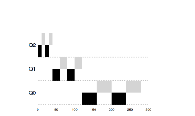
In this example, there are 2 tasks that worked in a high priority queue for 20
ms, divided into windows of 10 ms. 40ms in the middle queue (window at 20ms) and in the low priority
queue, the time window became 40ms, where the tasks completed their work.
The Solaris OS MLFQ implementation is a class of time-sharing schedulers.
The scheduler provides a set of tables that determine exactly how it should
the priority of the process changes over the course of its life, what the size of the
selected window should be, and how often it is necessary to raise the priorities of the task. The
system administrator can interact with this table and make the scheduler behave
differently. By default, this table has 60 queues with a gradual increase
in window size from 20ms (high priority) to several hundred ms (lowest priority), as
well as with a boost of all tasks once per second.
Other MLFQ planners do not use the table or any specific
rules that are described in this lecture; on the contrary, they calculate priorities using
mathematical formulas. So, for example, the scheduler in FreeBSD uses the formula for
calculating the current priority of the task, based on how much the process
used the CPU. In addition, the use of the CPU decays over time, and thus
increasing the priority occurs somewhat differently than described above. These are
called decay algorithms. Since version 7.1, FreeBSD uses the ULE scheduler.
Finally, many planners have other features. For example, some
schedulers reserve the highest levels for operating system operation and thus
, no user process can get the highest priority in the
system. Some systems allow you to give advice in order to help the
planner correctly prioritize. For example, using the nice command
You can increase or decrease the priority of the task and thus increase or
decrease the chances of the program for processor time.
MLFQ: Summary
We described a planning approach called MLFQ. Its name is
concluded in the principle of work - it has several queues and uses feedback
to determine the priority of the task.
The final form of the rules will be as follows:
- Rule1 : If priority (A)> Priority (B), task A will start (B will not)
- Rule2 : If priority (A) = Priority (B), A&B are started using RR
- Rule3 : When a task enters the system, it is queued with the highest priority.
- Rule4 : After the task has used up the time allotted to it in the current queue (regardless of how many times it freed up the CPU), the priority of such a task decreases (it moves down the queue).
- Rule5 : After a certain period of S, transfer all the tasks in the system to the highest priority.
MLFQ is interesting for the following reason - instead of demanding knowledge about the
nature of the task in advance, the algorithm examines the past behavior of the task and
prioritizes accordingly. Thus, he tries to sit on two chairs at once - to achieve productivity for small tasks (SJF, STCF) and honestly run long,
CPU-loading tasks. Therefore, many systems, including BSD and their derivatives,
Solaris, Windows, Mac, use some form of
MLFQ algorithm as a scheduler as a base.