Estimation of VaR and ConVaR for the stock price of the Kazakhstani company

The last decades the world economy regularly falls into this vortex of financial crises that have affected each country. It almost led to the collapse of the existing financial system, due to this fact, experts in mathematical and economic modelling have become to use methods for controlling the losses of the asset and portfolio in the financial world (Lechner, L. A., and Ovaert, T. C. (2010). There is an increasing trend towards mathematical modelling of an economic process to predict the market behaviour and an assessment of its sustainability (ibid). Having without necessary attention to control and assess properly threats, everybody understands that it is able to trigger tremendous cost in the development of the organisation or even go bankrupt.

Value at Risk (VaR) has eventually been a regular approach to catch the risk among institutions in the finance sector and its regulator (Engle, R., and Manganelli S., 2004). The model is originally applied to estimate the loss value in the investment portfolio within a given period of time as well as at a given probability of occurrence. Besides the fact of using VaR in the financial sector, there are a lot of examples of estimation of value at risk in different area such as anticipating the medical staff to develop the healthcare resource management Zinouri, N. (2016). Despite its applied primitiveness in a real experiment, the model consists of drawbacks in evaluation, (ibid).

The goal of the report is a description of the existing VaR model including one of its upgrade versions, namely, Conditional Value at Risk (CVaR). In the next section and section 3, the evaluation algorithm and testing of the model are explained. For a vivid illustration, the expected loss is estimated on the asset of one of the Kazakhstani company trading in the financial stock exchange market in a long time period. The final sections 4 and 5 discuss and demonstrate the findings of the research work.

Background

It is believed that the first usage of the VaR by the giant financial organisations up to 40 years ago and in consequence VaR has become popular among other trading firms, even financial regulators have had attention to the model (Linsmeier, T. J., and Pearson, N. D. 2000). For instance, the U.S. Securities and Exchange Commission inscribed VaR on a list of quantitative methods for calculating the market risk and property in 1997 (ibid).

Actually, according to articles of Lechner, L. A., and Ovaert, T. C. (2010) as well as Linsmeier, T. J., and Pearson, N. D. (2000), VaR is an estimating equation expressed in monetary units which do not exceed the loss in magnitude range during a given time period and given confidence level. Typically, the confidence level of the model estimation (99%, 97.5%, 95%) or in other words the probability that some unfavourable case will have happened and influence on the market are equal to 1, 2.5 and 5 percent (ibid).

The well-known equation of the VaR is able to be described (Phelps S, 2018):

Where X is a random variable that performs the amount of the portfolio’s value, and is a cumulative distribution function (ibid).

On the other hand, Hooper G.P. (1996, cited in Lechner, L. A., and Ovaert, T. C. 2010) denotes VaR with confidence alpha defines in a quite elementary way:

Where $$ is the standard deviation of selected stock returns, $$ is the square root of the fixed time period and $$ is the cumulative distribution function (CDF) for a normal distribution (Lechner, L. A., and Ovaert, T. C. 2010).

Although VaR is a well-known and handled method to estimate decided portfolio risk, there are shortcomings in a case when measuring vulnerability to ultimate market issues, namely, the example is related to the probability of extreme market events is not adequately caught in the tail of the normal distribution (Capiński, M. J. 2015). To solve this issue, the Conditional Value at Risk (CVaR) was created which consider the expected value of loss instead of VaR (ibid). CVaR defines as:

Where Ahn D.-H. et.al (1999, cited in Capiński, M. J. 2015) interpret $$
as VaR of X random variable (return of a stock price) with probability $$ and defines as the upper quantile of X.

Moreover, Acerbi C. and Tasche D. (2002, cited in Capiński, M. J. 2015) confirm, “The CVaR is a coherent risk measure”. Rockafellar, R. T., and Uryasev, S. (2000) notice that CVaR has extra features: transition-equivariant, positively homogeneous, convex and etc.

The following chapter of the article demonstrates the implementation of wellknown Value at Risk (VaR) and Conditional Value at Risk (CVaR) also announced as Expected shortfall (ES) noticed in the work of Rockafellar, R. T., and Uryasev, S. (2000) by using information technology on real data.

Methodology

Let consider the most commonly used methods for calculating VaR, as well as its advantages and disadvantages.

According to the report of Lechner, L. A., and Ovaert, T. C. (2010), the historical simulation is a widespread approach to evaluate VaR and its modification. In historical modelling of the data, we take the values of financial fluctuations for the portfolio which are already known from past measurements. It is therefore only logical sequence that the disadvantage of this method is the impossibility of building predictions for portfolios without a piece of information about it. The Monte Carlo method is in many ways identical to the method of historical modelling that used for high-accurate technique, the main clear difference that the calculation of Monte Carlo simulation is not based on real data, but realized on randomly generated values. The advantage of this method is the possibility of considering as a large number of situations, and emulating market behaviour in extreme conditions as well as there is no need an approximation between risk factors and changes in a portfolio (Glasserman, P., Heidelberger, P. and Shahabuddin, P., 2002). The obvious drawback is the large computational resources required to implement this approach (ibid).

Naturally, these are not the only these methods for calculating VaR models. In addition, there are both simple linear and quadratic models of price prediction, and a rather complicated method of variations, which were not covered in the essay.

Data analysis

As secondary data for testing the accurate estimation, the stock of KAZ Minerals is taken. To be clarified the work, the Adjusted closed price is taken for simulation in a model. The shares of KAZ Minerals company (KAZ.L) is one the successfully trading securities among Kazakhstani firms on the London Stock Exchange (LSE) as well as categorized in Premium Equity Commercial Companies list (London Stock Exchange, 2019). The entity presents itself as the massive copper mining company in Kazakhstan (Kazminerals.com. 2019).

The historical data of the share price is downloaded from Yahoo Finance web site (Finance.yahoo.com, 2019). To ensure the validity of the work, the period of one year from 22 March 2018 to 22 March 2019 is observed. Furthermore, to avoid the information disruption, in the analysis, the historical data of the KAZ.L share price is downloaded in Comma-Separated Values (CSV) format due to the fact that the CSV format is compatible by Microsoft Excel program (Excel). The chosen data of the project is presented as a line graph by using Excel in Figure 1.

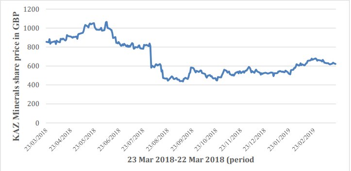
Figure 1. The dynamic of change KAZ Minerals stock price for one year

Owing to the limitation of the report timeline, instead of using a programming language like Python for implementation of assessment models, the data is analysed completely in Excel.

Findings

In the previous section, the models to forecast the potential losses in a portfolio based on VaR and CVaR equation and used changes in KAZ Minerals share price from 23 March 2018 to 23 March 2019, downloaded from official web source Yahoo Finance (Finance.yahoo.com, 2019). Both equations executed for each date from the chosen period.

Table 1 demonstrates the mean business daily return, a standard deviation of returns, a minimum value of returns and a maximum value of returns for this example.

Table 1. Share mean return and standard deviation of returns

The corresponding mean is -0.0006 and standard deviation 0.0355 of the returns for the selected unique security KAZ Minerals. What is more that the variance of the returns is 0.0013. Additionally, that should certainly be underlined that in the research work of Vee, D. N. C., and Gonpot, P. N (2014) the Kazakhstani stock returns showed considerable value in volatility however the estimation was related to the index of Kazakhstan Stock Exchange in pre and post period 2008. Also, it should be mentioned that the maximum value among returns is 0.0998, as well as the minimum value among returns is -0.2829 in loss distribution. Table 2 presents the maximum and minimum values among Adjusted close stock price(KAZ.L) in Pound Sterling (GBP) trading in London Stock Exchange from 23 March 2018 to 22 March 2019.

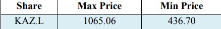
Table 2. The maximum and minimum KAZ Minerals stock price in GBP

The following step is evaluation Value at Risk (VaR) and Conditional Value at Risk (CVaR) for the confidence level — 0.99, 0.972 and 0.95. The values are revealed in Table 3.

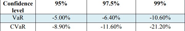
Table 3. VaR and CVaR values of the returns

The sample size of the simulation is taken 252 units from 23 March 2018 to 22 March 2019 during one year.

Discussion

In the report, VaR and CVaR equations demonstrate the credible value in case of the estimation models for a share price of Kazakhstani company in the short-term period. With these values at one hand, both methods present adequate results to assess the value of the threats for investment portfolio (Linsmeier, T. J., and Pearson, N. D. 2000; Lechner, L. A., and Ovaert, T. C. 2010).

Moreover, according to findings from Table 2, the next notice is straightforward that the values for CVaR are more massive in comparison with the VaR values by all confidence level measures. It can be given an explanation by the fact the CVaR takes chosen portfolio average risk consequently it is more sensitive on the tail of the loss distribution than VaR. This proves once again that CVaR is a coherent risk (Acerbi C. and Tasche D., 2002, cited in Capiński, M. J. 2015; Rockafellar, R. T., and Uryasev, S. 2000). For example, with regard to the adequacy of both estimation models, with confidence level 99% VaR and CVaR illustrate the significant per cent of loss from returns of the stock. To be precise, it might be detected VaR is -10.60% and CVaR is -21.20%. It is pretty clear the reason of the colossal measures of CVaR with a given confidence level 99% due to the fact the range of stock price during the period, the maximum price is 1065.06 GBP minimum stock price is 436.70 GBP, respectively.

Conclusion

Having considered everything above, it should be obviously mentioned again that the aim of the report is to demonstrate the estimation of the value of possible loss for Kazakhstani company (KAZ Minerals) over a period from 23 March 2018 to 22 March 2019. The evaluation methods formed on Value at Risk (VaR) and Conditional Value at Risk (CVaR) equations. The performances from the simulation are compared to each other in the same time period. The results show the significant value for each method and prove the previous work on the same area that CVaR has more accurate measures in comparison with VaR (Acerbi C. and Tasche D., 2002, cited in Capiński, M. J. 2015; Rockafellar, R. T., and Uryasev, S.2000).

Despite criticism, VaR a widespread tool in all financial institutions to present day and there are a wide range of its modification version. Owing to the obstacles of the complex calculation in the deep research, the experiment is done by using Microsoft Excel instead of using a programming language like Python, as well as the results are revealed in the report. The results of the essay are able to be a basement for further work in using complex estimation measure of risk for the portfolio in the stock exchange industry, the insurance industry and investment industry.