How we overclocked CAD COMPASS-3D → Part 2
In the last part, we talked about the birth of KOMPAS-3D v18, something about the selection of criteria and models for testing new functions, and also touched on the topic of rendering in the “Basic” version.
Let's continue with the story about the “Improved” rendering option.

The script with the addition of components to a large assembly eventually developed into the so-called complex test, which is described in Table 2.
Table 2. Scenario with the addition of components to a large assembly. Test criteria.
In the table you can see the points (drawing, opening), which from the very beginning were selected as separate directions of accelerations. But improvements required other components.
Significant time was taken by synchronization with a tree. We solved the problem by implementing a partial update.
Another difficulty was the significant impact of the specification on the performance of KOMPAS-3D. In some complex test scenarios, this component was the main one (50% or more).
Add components to the assembly “Reducer of the ship’s power plant”.
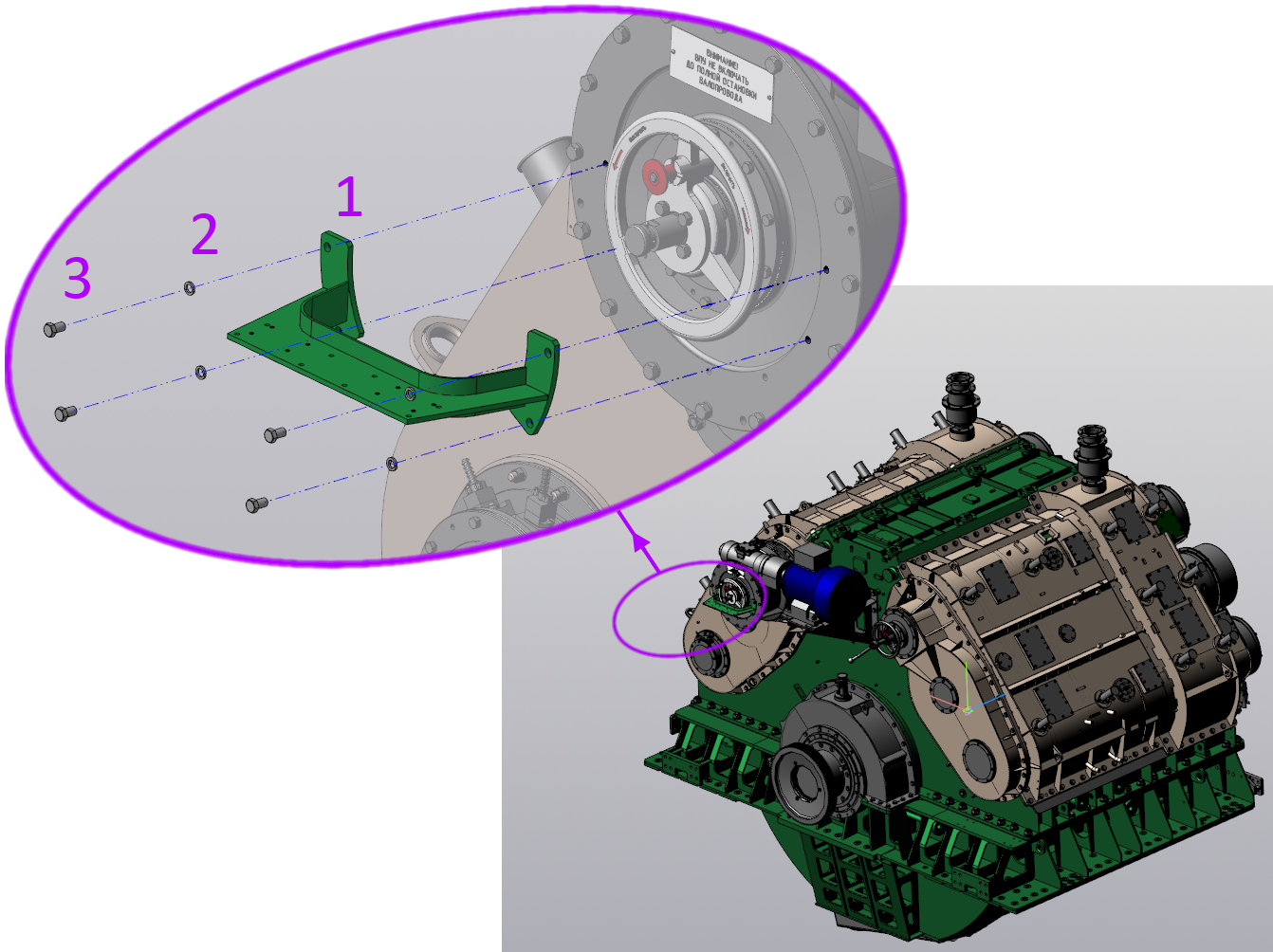
Comprehensive test for the assembly "Reducer of a marine power plant."
The numbers show: 1 - bracket, 2 - washer, 3 - bolt.
Table 3. Insertion time of components in a large assembly in seconds. Less is better.
A comprehensive test can be considered as one of the editing scenarios of the assembly (from the number of common ones).
In addition, assembly rebuilding accelerated. Now, if you edit an operation, the entire assembly will not be completely rebuilt - only the changed objects will be updated. To determine the dependent operations, that is, those operations, the result of which could be affected by the result of the changed operation, a special algorithm is used that builds connections between operations, bodies and inserts.
The main idea to increase the speed of reading files is to make KOMPAS-3D read only what the user needs at the moment.
For instance:
All this required refinement of the data structure in the file so that its individual parts could be read.
Based on the improvements, a new type of assembly loading appeared - “Partial”. In this type of loading, only results (bodies, surfaces) and triangulation are subtracted from the file. Partial loading allows you to create pairings and is close in terms of functionality to the full loading of components.
After implementing improvements on partial reading, the creation of custom loading types becomes promising.
For components that are not important for future builds, the “Empty” load type can be applied. These may be components hidden inside others (“vnutryanka”). In v18, components (and entire assemblies) with the “Empty” boot type open almost instantly.
Table 4. Opening times for assemblies with the “Empty” and “Dimension” boot types in seconds. Less is better.
The remaining components, which are needed to understand the appearance of the product or will be used as supporting objects for further construction, can be loaded “Full” or “Partially”.
As a tool for preparing custom boot types, you can use new commands to select “invisible” components. We apply the command and then use the context menu to change the type of loading for the selected components to “Empty”.
When accelerating projection, we asked ourselves the question of filtering the data received at the input of the mathematical core.
First of all, we decided to filter invisible components / bodies. For this purpose, the occlusion-culling mechanism was used - it allows you to find out if the body that will be projected is visible or it closes and is inside some other body. This operation is performed on the side of the video card.
The greatest effect will be when creating projections of models with a large number of components hidden inside closed volumes, for example:
For inclusion, the option "Rough projection" is responsible. The name is not accidental - relatively small parts (for example, a bolt at the scale of a power plant) may not be projected on an assembly scale. For many users, this state of affairs will suit, especially in the case of creating dimensional drawings and general drawings.
Even without using this option, projection is noticeably faster compared to V16 and v17. This was helped by improvements on the side of the mathematical core.
Table 5. Time to create three standard projections in seconds. Less is better.
Also in v18, the possibility of rebuilding individual associative species was implemented.
In a drawing containing many associative views, the user has the opportunity to rebuild individual irrelevant views. For example, the one to which he wants to add annotations. You can also specify the views built with the Rough Projection option enabled.
This feature does not apply to explicit accelerations, but allows the user to save time.
The result of the work done to accelerate the projection of the model Vacuum-technological installation in the drawing:
In the next part, we will describe how we accelerated the calculation of mass-centering characteristics (MTC), about the contribution of the c3dlabs geometric core to COMPAS-3D performance , changes to C3D Modeler, and also about which hardware is suitable for v18.
Let's continue with the story about the “Improved” rendering option.
Drawing calls
Below we present the results of the rendering speed during assembly rotation. Recall that 24 frames per second (fps) are considered to be comfortable indicators for the human eye.Alexander Tulup, programmer:
“The main problem of the performance of displaying large scenes is associated with a large number of so-called“ drawing calls ”. The old version of the rendering is built on top of the mathematical data model. Thus, for each primitive - points, edges, faces - a separate method was called for its display.
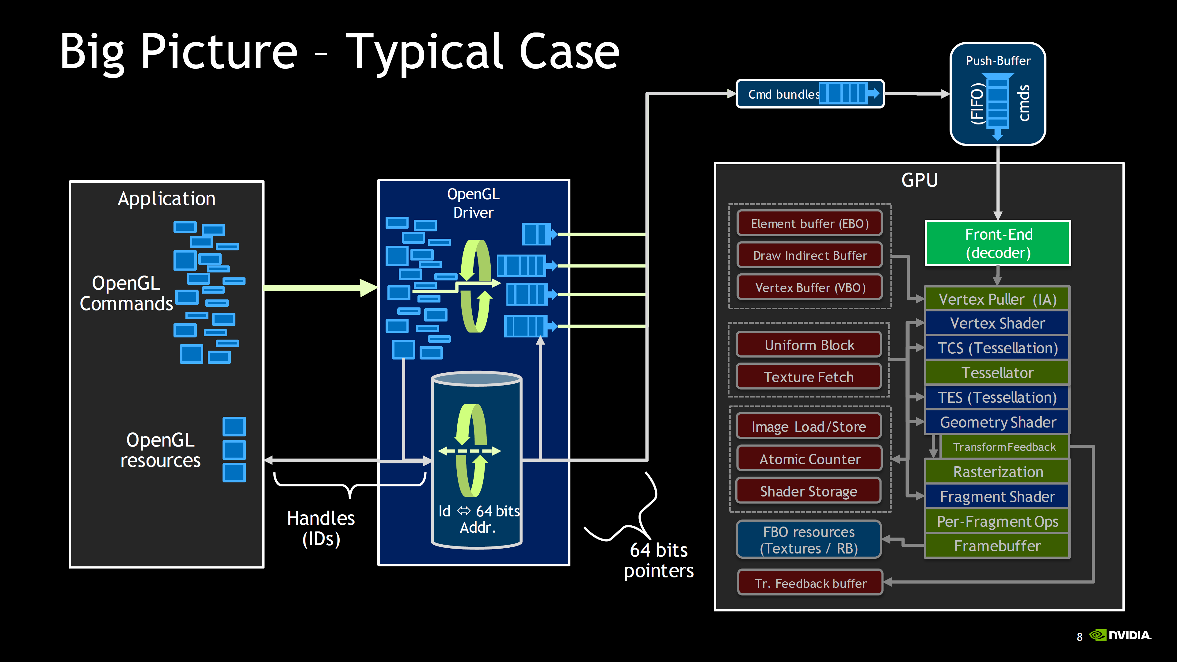
For each draw call, OpenGL (driver) performs a series of checks, simultaneously translating the incoming commands into a format that the video card understands, after which the calls are added to the queue and are already sent for execution.
GPU command transfer scheme in OpenGL ( source )
With a large number of details, the number of calls to the CPU grows so much that the data simply does not have time to arrive on the video card. We get a situation where on a very strong video card it “slows down” in the same way as on a medium or weaker one.
You can deal with this by reducing the number of renderings (state transitions) - group by material, combine common geometry ( instancing ), etc.
We should not forget that from the whole scene we see only some of it. Algorithms for detecting invisible objects (frustum culling, occlusion culling, etc.) are applicable here,
inspired by the example of The Road to One Million Draws and AZDO, we decided to go in a rather unusual way: get rid of the state transition on the CPU side as much as possible. Now almost everything is done on the graphics card. All the necessary attributes are taken directly from the video memory while drawing from the shader itself ( shader ), which was made possible thanks to the increase in video memory ( VRAM ) and the advent of SSBO .
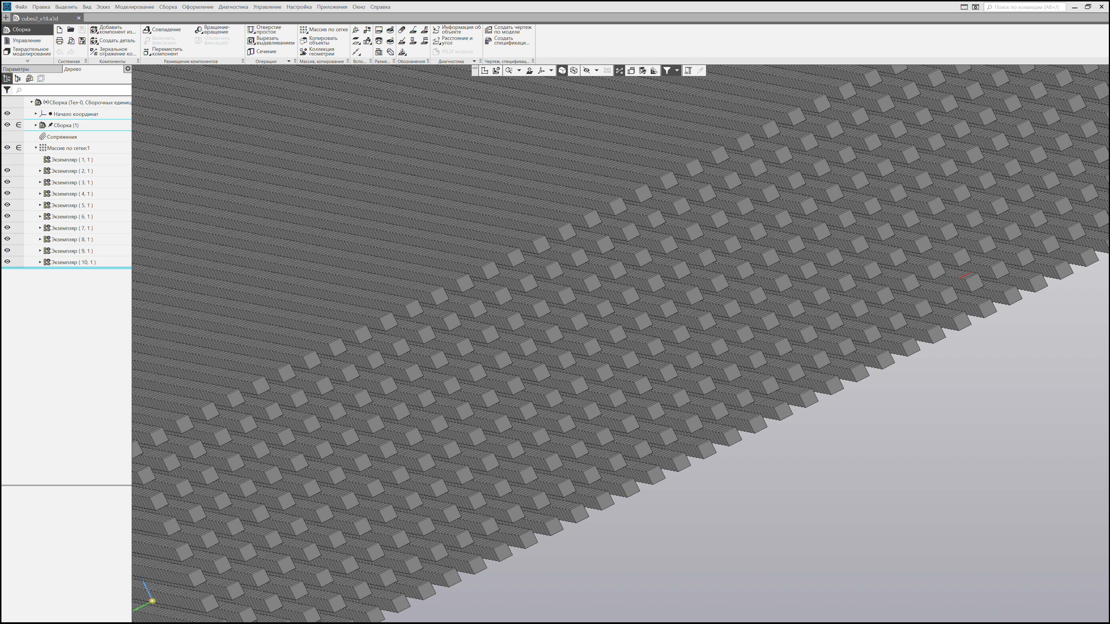
1,000,000 dice
Of the advantages of this approach: the display speed has become really high. Speed is limited only by the capabilities of the GPU, namely the amount of data that it is able to process.
It also allowed quite efficiently implement clipping mechanisms for invisible objects. The results of the visibility check are recorded directly in the video memory, and from there the drawing commands are formed based on them. That is, on the CPU side, you do not need to wait.
One of the main disadvantages of this approach is the high complexity of development. Much has to be implemented anew, taking into account the chosen approach. In addition, we often had to deal with a situation where the same shader code worked differently or did not work at all on video cards from different manufacturers. Often this was "treated" by updating the driver, but sometimes after a long debugging it was necessary to rewrite the code.
Naturally, the requirements for the video card also increased. Support for OpenGL 4.5 is a key, but not the only requirement.

Hereinafter, measurements were taken on a PC with the following configuration:Table 1. Frame rate (frames per second, fps) on various models. More is better. Display mode: Halftone + wireframe, simplified mode disabled, anti-aliasing quality: medium (MSAA 8x)
CPU: Intel Core i7-6700K 4.00 GHz
RAM: 32 Gb
GPU: NVidia Quadro P2000
OS: Microsoft Windows 10 x64 Professional
| Model | Number of components | Frame rate, fps | ||
| V16.1 | v17.1 | v18 | ||
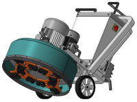 Mosaic grinding machine | 2764 | 4.1 | 4.7 | 124.9 |
 PGU-410 | 108337 | 0.3 | 0.4 | 28.6 |
 Car dumper | 17342 | 1,1 | 1.4 | 124.7 |
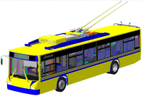 Trolley bus | 9783 | 1.9 | 2,4 | 124.9 |
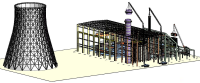
 Northern Tidal Power Station | 48445 | 0.3 | 0.5 | 76.1 |
 Vacuum technological installation | 7189 | 1.9 | 2,3 | 124.9 |
 Marine power plant gearbox | 6414 | 2.6 | 3.6 | 123.9 |
Adding Components to a Large Assembly
The script with the addition of components to a large assembly eventually developed into the so-called complex test, which is described in Table 2.
Table 2. Scenario with the addition of components to a large assembly. Test criteria.
| Criterion | Criterion Description |
| File open speed | The component added to the assembly must be loaded from disk |
| Render speed | The assembly and the inserted component must be positioned, for this you need to rotate / move / zoom the image |
| Object selection speed | To create mates, you need to select the basic objects: faces, planes, edges, etc. |
| Synchronization speed with the build tree | The component added to the assembly and its interfaces must be represented in the construction tree |
| Specification Module Sync Speed | The component added to the assembly must be considered in the specification. |
In the table you can see the points (drawing, opening), which from the very beginning were selected as separate directions of accelerations. But improvements required other components.
Significant time was taken by synchronization with a tree. We solved the problem by implementing a partial update.
Another difficulty was the significant impact of the specification on the performance of KOMPAS-3D. In some complex test scenarios, this component was the main one (50% or more).
Specification
The specification is the KOMPAS-3D system module, which is responsible for the formation of the design document of the same name. It is developed by a separate team.
In particular, the team accelerated synchronization during insertion by redesigning the internal mechanisms of the specification module.
Some results
Add components to the assembly “Reducer of the ship’s power plant”.
Comprehensive test for the assembly "Reducer of a marine power plant."
The numbers show: 1 - bracket, 2 - washer, 3 - bolt.
Table 3. Insertion time of components in a large assembly in seconds. Less is better.
| Component | Act | Time s | |||
| V16.1 | v17.1 | v18 | |||
Component Insert Bracket 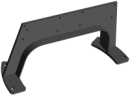 | Loading | 2.0 | 3.0 | 2.2 | |
| Switch to pairing mode | 0.6 | 0.4 | 0.4 | ||
| First pairing | First Object Selection | 0.4 | 1,0 | 0.2 | |
| The choice of the second object | 0.5 | 1,1 | 0.2 | ||
| Select the right pairing | 3.8 | 3.6 | 1,0 | ||
| Second pairing | First Object Selection | 0.5 | 1.4 | 0.5 | |
| The choice of the second object | 0.5 | 1.4 | 0.2 | ||
| Select the right pairing | 3.6 | 3.0 | 1,2 | ||
| Third pairing | First Object Selection | 0.5 | 0.5 | 0.5 | |
| The choice of the second object | 0.3 | 1,1 | 0.3 | ||
| Select the right pairing | 3,7 | 3.2 | 1,1 | ||
| Confirm Insert Creation | 7.8 | 5.2 | 2,3 | ||
| Total Bracket Insert | 24.2 | 24.6 | 10.1 | ||
| Insert a washer from the standard product library  | First pairing selection | 6.4 | 2,4 | 0.4 | |
| Second pair selection | 4.2 | 3,1 | 0.4 | ||
| Confirm Insert Creation | 15.7 | 9.2 | 4.4 | ||
| Total for Insert Washers | 26.3 | 14.7 | 5.2 | ||
Bolt insert 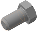 | Loading | 2.0 | 2.7 | 2.0 | |
| Switch to pairing mode | 0.5 | 0.5 | 0.5 | ||
| First pairing | First Object Selection | 0.4 | 1,0 | 0.2 | |
| The choice of the second object | 0.4 | 1,1 | 0.2 | ||
| Select the right pairing | 3.4 | 2.7 | 1,0 | ||
| Second pairing | First Object Selection | 0.4 | 1,2 | 0.4 | |
| The choice of the second object | 0.5 | 0.5 | 0.4 | ||
| Select the right pairing | 3,7 | 2.9 | 1,0 | ||
| Third pairing | First Object Selection | 0.5 | 1,0 | 0.5 | |
| The choice of the second object | 0.5 | 1,0 | 0.2 | ||
| Select the right pairing | 4.2 | 3.9 | 1,2 | ||
| Confirm Insert Creation | 32,5 | 5,4 | 2.2 | ||
| Total for Bolt insertion | 49 | 21,2 | 9.8 | ||
| The total insertion of the three components | 99.5 | 60.5 | 25.1 | ||
A comprehensive test can be considered as one of the editing scenarios of the assembly (from the number of common ones).
In addition, assembly rebuilding accelerated. Now, if you edit an operation, the entire assembly will not be completely rebuilt - only the changed objects will be updated. To determine the dependent operations, that is, those operations, the result of which could be affected by the result of the changed operation, a special algorithm is used that builds connections between operations, bodies and inserts.
Opening assemblies
The main idea to increase the speed of reading files is to make KOMPAS-3D read only what the user needs at the moment.
For instance:
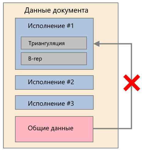
- read only current execution for assembly inserts,
- for download types, read only the necessary information: triangulation or triangulation + results ( B-rep ).
All this required refinement of the data structure in the file so that its individual parts could be read.
In addition to accelerating the opening of files, partial reading also helped to reduce the resources consumed - primarily RAM.Anton Sidyakin, programmer, teamlead:
“For some time now, the KOMPAS-3D file has been an archive combining several service files. One of them contains model / assembly document data organized in a tree structure. The ability to navigate this structure already existed. For partial reading, it was necessary to ensure the independence of the parts from each other. Thus, the parts received should not have referred to each other, otherwise the part with the link would have become “inferior”.
As a result, for details, it was possible to separate the performance from the document and from each other. In assemblies, the container for inserts and mates is highlighted separately. Inside the executions, it was also possible to separate the initial data for the construction and the results in the form of triangulation and bodies.
If we talk about simplified types of loading, then the editable assembly is fully loaded, and only triangulation and, depending on the type, boundary representation (B-rep) are loaded from its inserts. Displaying inserts with changed external variables in this mode presented some difficulties, since they were previously obtained on the fly by rebuilding while reading, and in simplified types of loading there is no data for this. The solution was to write down the results of rebuilding such inserts into the assembly. This gave acceleration and due to the lack of rebuilding.
The described division of the document into parts allowed loading into the assembly only the performances selected in the inserts.

Based on the improvements, a new type of assembly loading appeared - “Partial”. In this type of loading, only results (bodies, surfaces) and triangulation are subtracted from the file. Partial loading allows you to create pairings and is close in terms of functionality to the full loading of components.
After implementing improvements on partial reading, the creation of custom loading types becomes promising.
hint
Custom boot types are combinations of system methods for loading a component. This function is not new, but improvements made in v18 allow you to get significant bonuses from its use.
For components that are not important for future builds, the “Empty” load type can be applied. These may be components hidden inside others (“vnutryanka”). In v18, components (and entire assemblies) with the “Empty” boot type open almost instantly.
Table 4. Opening times for assemblies with the “Empty” and “Dimension” boot types in seconds. Less is better.
| Model | Download Type | Opening time, s | ||
| V16.1 | v17.1 | v18 | ||
Vacuum technological installation | Empty | 12.8 | 11.7 | 2,5 |
| Size | 21,2 | 20.8 | 2.6 | |
Marine power plant gearbox | Empty | 31,0 | 15.9 | 7.2 |
| Size | 371.5 | 114.8 | 7.3 | |
The remaining components, which are needed to understand the appearance of the product or will be used as supporting objects for further construction, can be loaded “Full” or “Partially”.
As a tool for preparing custom boot types, you can use new commands to select “invisible” components. We apply the command and then use the context menu to change the type of loading for the selected components to “Empty”.
Projection
When accelerating projection, we asked ourselves the question of filtering the data received at the input of the mathematical core.
First of all, we decided to filter invisible components / bodies. For this purpose, the occlusion-culling mechanism was used - it allows you to find out if the body that will be projected is visible or it closes and is inside some other body. This operation is performed on the side of the video card.
The greatest effect will be when creating projections of models with a large number of components hidden inside closed volumes, for example:
- complex drives, gearboxes, etc.,
- vehicles
- buildings
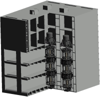
- cabinets with electrical equipment.
For inclusion, the option "Rough projection" is responsible. The name is not accidental - relatively small parts (for example, a bolt at the scale of a power plant) may not be projected on an assembly scale. For many users, this state of affairs will suit, especially in the case of creating dimensional drawings and general drawings.
Read more about the Rough Projection option.
The option is available only for standard projections. For specifying images (sections, sections, remote views) "Rough projection" is not involved.
Even without using this option, projection is noticeably faster compared to V16 and v17. This was helped by improvements on the side of the mathematical core.
Table 5. Time to create three standard projections in seconds. Less is better.
| Model | Time to create three standard projections, s | |||
| V16.1 | v17.1 | v18 Included rough projection | v18 Disabled rough projection | |
Vacuum technological installation | 124.1 | 47.5 | 12.9 | 34.6 |
Marine power plant gearbox | 256 | 410 | 38,4 | 54,4 |
 Multipurpose Unified Box Body | 99.9 | 123,4 | 44.9 | 53.5 |
Also in v18, the possibility of rebuilding individual associative species was implemented.
In a drawing containing many associative views, the user has the opportunity to rebuild individual irrelevant views. For example, the one to which he wants to add annotations. You can also specify the views built with the Rough Projection option enabled.
Rebuild a single view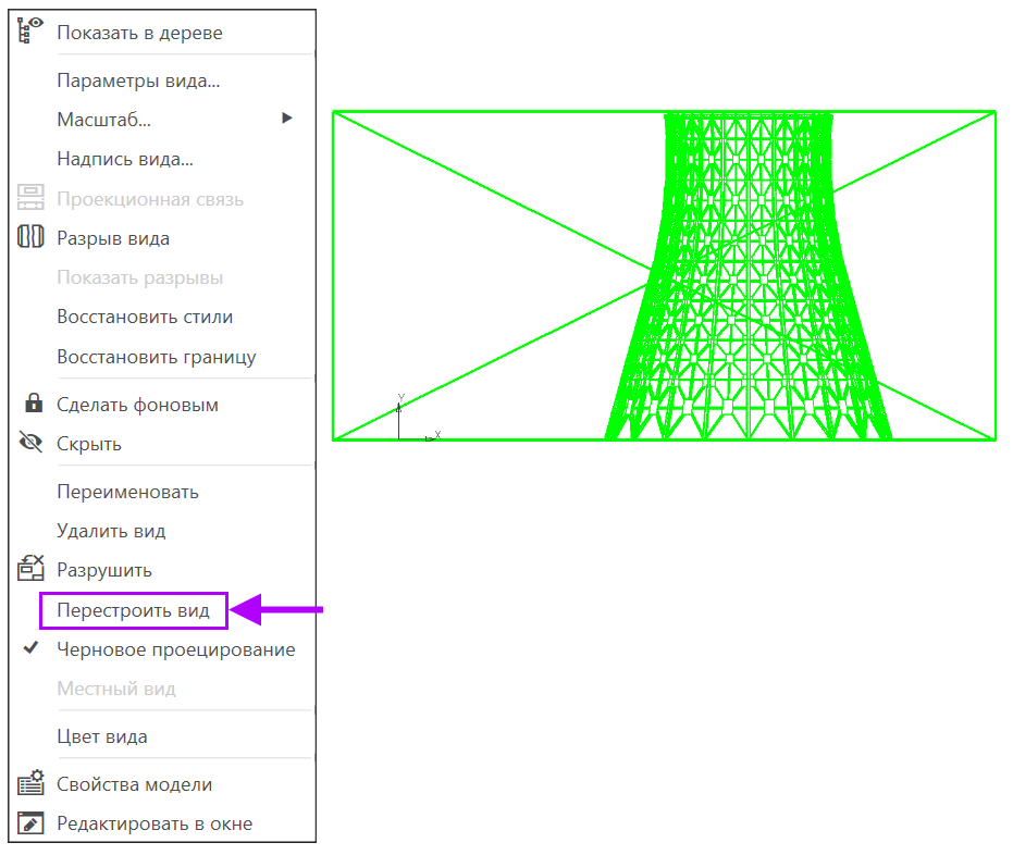
This feature does not apply to explicit accelerations, but allows the user to save time.
The result of the work done to accelerate the projection of the model Vacuum-technological installation in the drawing:
In the next part, we will describe how we accelerated the calculation of mass-centering characteristics (MTC), about the contribution of the c3dlabs geometric core to COMPAS-3D performance , changes to C3D Modeler, and also about which hardware is suitable for v18.