Ensemble methods. Excerpt from a book

Hi, Khabrozhiteli, we have handed over to the printing house a new book “Machine Learning: Algorithms for Business” . Here is an excerpt about ensemble methods, its purpose is to explain what makes them effective, and how to avoid common mistakes that lead to their misuse in finance.

6.2. Three sources of error

MO models usually suffer from three errors .

1. Bias: this error is caused by unrealistic assumptions. When the bias is high, this means that the MO algorithm could not recognize the important relationships between the traits and outcomes. In this situation, it is said that the algorithm is "unapproved."

2. Dispersion: this error is caused by sensitivity to small changes in the training subset. When the variance is high, this means that the algorithm is overfitted to the training subset, and therefore even minimal changes in the training subset can produce terribly different predictions. Instead of modeling general patterns in a training subset, the algorithm mistakenly takes noise for the signal.

3. Noise: This error is caused by the dispersion of the observed values, such as unpredictable changes or measurement errors. This is a fatal error that cannot be explained by any model.


An ensemble method is a method that combines many weak students, who are based on the same learning algorithm, with the goal of creating a (stronger) student whose performance is better than any of the individual students. Ensemble techniques help reduce bias and / or dispersion.

6.3. Bootstrap Aggregation

Bagging (aggregation), or aggregation of bootstrap samples, is an effective way to reduce the variance in forecasts. It works as follows: first, it is necessary to generate N training subsets of data using random sampling with return. Second, fit N evaluators, one for each training subset. These evaluators are adjusted independently of each other, therefore, models can be adjusted in parallel. Thirdly, the ensemble forecast is a simple arithmetic mean of individual forecasts from N models. In the case of categorical variables, the probability that an observation belongs to a class is determined by the share of evaluators who classify this observation as a member of this class (by majority vote, that is, by a majority vote).

If you use the sklearn library's BaggingClassifier class to calculate non-packet accuracy, then you should be aware of this defect: https://github.com/scikit-learn/scikitlearn/issues/8933 . One workaround is to rename labels in an integer sequential order.

6.3.1. Dispersion reduction

The main advantage of bagging is that it reduces the variance of forecasts, thereby helping to solve the problem of overfitting. The variance in the bagged prediction (φi [c]) is a function of the number of bagged appraisers (N), the average variance of the prediction performed by one appraiser (σ̄), and the average correlation between their predictions (ρ̄):


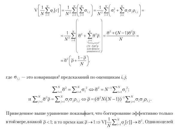
sequential bootstraping (chapter 4) is to take samples as independent as possible, thereby reducing ρ̄, which should reduce the dispersion of bagged classifiers. In fig. 6.1, we plotted the standard deviation diagram of the bagged prediction as a function of N ∈ [5, 30], ρ̄ ∈ [0, 1], and σ̄ = 1.

6.3.2. Improved accuracy

Consider a bagged classifier, which makes prediction on k classes by a majority vote among N independent classifiers. We can designate predictions as {0,1}, where 1 means correct prediction. The accuracy of the classifier is the probability p to mark the prediction as 1. On average, we get Np predictions marked as 1 with a variance of Np (1 - p). The majority vote makes the correct prediction when the most predictable class is observed. For example, for N = 10 and k = 3, the bagged classifier made the correct prediction when observed



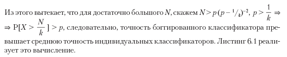
Listing 6.1. The correctness of the bagged classifier

from scipy.misc import comb
N,p,k=100,1./3,3.
p_=0
for i in xrange(0,int(N/k)+1):
     p_+=comb(N,i)*p**i*(1-p)**(N-i)
print p,1-p_

This is a strong argument in favor of bagging any classifier in the general case, when computational capabilities allow it. However, unlike boosting, bagging cannot improve the accuracy of weak classifiers:


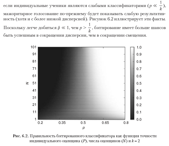
For a detailed analysis of this topic, the reader is advised to turn to the Condorcet jury theorem. Although this theorem was obtained for the purpose of majority voting in political science, the problem addressed by this theorem has common features with the one described above.

6.3.3. Redundancy of observations

In Chapter 4, we examined one of the reasons financial observations cannot be considered equally distributed and mutually independent. Excessive observations have two detrimental effects on bagging. Firstly, samples taken with return are more likely to be almost identical, even if they do not have common observations. It doesand bagging will not reduce the variance, regardless of N. For example, if each case at t is marked in accordance with a financial return between t and t + 100, then we must select 1% of cases per bagged appraiser, but no more. In chapter 4, section 4.5, three alternative solutions are recommended, one of which was setting max_samples = out ['tW']. Mean () in the implementation of the bagged classifier class in the sklearn library. Another (better) solution was the application of the method of sequential bootstrap selection.

The second detrimental effect of observation redundancy is that extra-packet accuracy will be inflated. This is due to the fact that random sampling with sampling returns to the training subset samples that are very similar to those outside the package. In this case, the correct stratified k-block cross-validation without shuffling before splitting will show much less accuracy on the test subset than that which was evaluated outside the package. For this reason, when using this sklearn library class, it is recommended to set stratifiedKFold (n_splits = k, shuffle = False), cross-check the bagged classifier, and ignore the results of non-packet accuracy. A low number of k is preferable to a high one, since over-partitioning will again place patterns too similar to those in the test subset.

6.4. Random forest

Decision trees are well known in that they tend to over-fit, which increases the variance of forecasts. In order to address this problem, a random forest (RF) method was developed to generate ensemble forecasts with lower variance.

A random forest has some common similarities with bagging in the sense of training individual evaluators independently on bootstraped data subsets. A key difference from bagging is that a second level of randomness is built into random forests: during optimization of each nodal fragmentation, only a random subsample (without returning) of attributes will be evaluated in order to further decorrelate the evaluators.

Like bagging, a random forest reduces the variance of forecasts without overfitting (recall that until). The second advantage is that a random forest evaluates the importance of attributes, which we will discuss in detail in Chapter 8. The third advantage is that a random forest provides estimates of off-package accuracy, however in financial applications they are likely to be inflated (as described in Section 6.3.3). But like bagging, a random forest will not necessarily exhibit lower bias than individual decision trees.

If a large number of samples is redundant (not equally distributed and mutually independent), there will still be a re-fit: random sampling with return will build a large number of almost identical trees (), where each decision tree is overfitted (a drawback due to which decision trees are notorious) . Unlike bagging, a random forest always sets the size of bootstrap samples according to the size of the training subset of data. Let's look at how we can solve this problem of re-fitting random forests in the sklearn library. For illustration purposes, I will refer to the sklearn library classes; however, these solutions can be applied to any implementation:

1. Set the max_features parameter to a lower value to achieve discrepancy between the trees.

2. Early stop: set the regularization parameter min_weight_fraction_leaf to a sufficiently large value (for example, 5%) so that the off-packet accuracy converges to out-of-sample (k-block) correctness.

3. Use the BaggingClassifier evaluator on the base DecisionTreeClassifier evaluator, where max_samples is set to average uniqueness (avgU) between samples.

• clf = DecisionTreeClassifier (criterion = 'entropy', max_features = 'auto', class_weight = 'balanced')
• bc = BaggingClassifier (base_estimator = clf, n_estimators = 1000, max_samples = avgU, max_features = 1.)

4. Use the BaggingClassifier evaluator on the base RandomForestClassifier evaluator, where max_samples is set to average uniqueness (avgU) between samples.

• clf = RandomForestClassifier (n_estimators = 1, criterion = 'entropy', bootstrap = False, class_weight = 'balanced_subsample')
• bc = BaggingClassifier (base_estimator = clf, n_estimators = 1000, max_samples = avgU, max_features = 1.)

5. Modify the random forest class to replace standard bootstraps with sequential bootstraps.

To summarize, Listing 6.2 shows three alternative ways to configure a random forest using different classes.

Listing 6.2. Three ways to set up a random forest

clf0=RandomForestClassifier(n_estimators=1000, class_weight='balanced_
                                        subsample', criterion='entropy')
clf1=DecisionTreeClassifier(criterion='entropy', max_features='auto',
                                        class_weight='balanced')
clf1=BaggingClassifier(base_estimator=clf1, n_estimators=1000,
                                        max_samples=avgU)
clf2=RandomForestClassifier(n_estimators=1, criterion='entropy',
                                        bootstrap=False, class_weight='balanced_subsample')
clf2=BaggingClassifier(base_estimator=clf2, n_estimators=1000,
                                        max_samples=avgU, max_features=1.)

When fitting decision trees, the rotation of the feature space in the direction coinciding with the axes, as a rule, reduces the number of levels necessary for the tree. For this reason, I suggest that you fit a random tree on the PCA of attributes, as this can speed up the calculations and slightly reduce the re-fit (more on this in Chapter 8). In addition, as described in Chapter 4, Section 4.8, the argument class_weight = 'balanced_subsample' will help prevent trees from misclassifying minority classes.

6.5. Boost

Kearns and Valiant [1989] were among the first to ask if weak valuers could be combined in order to achieve the realization of a highly accurate valuer. Shortly afterwards, Schapire [1990] showed an affirmative answer to this question using a procedure that we call boosting today (boosting, boosting, amplification). In general terms, it works as follows: first, generate one training subset by random selection with return in accordance with certain sample weights (initialized by uniform weights). Secondly, fit one evaluator using this training subset. Thirdly, if a single appraiser achieves accuracy that exceeds the acceptability threshold (for example, in a binary classifier, it is 50%, so that the classifier works better, than random fortune telling), the evaluator remains, otherwise he is discarded. Fourth, give more weight to incorrectly classified observations and less weight to correctly classified observations. Fifth, repeat the previous steps until N appraisers are received. Sixth, the ensemble forecast is the weighted average of individual forecasts from N models, where weights are determined by the accuracy of individual evaluators. There are a number of boosted algorithms, of which AdaBoost adaptive boosting is one of the most popular (Geron [2017]). Figure 6.3 summarizes the decision flow in the standard implementation of the AdaBoost algorithm. give more weight to incorrectly classified observations and less weight to correctly classified observations. Fifth, repeat the previous steps until N appraisers are received. Sixth, the ensemble forecast is the weighted average of individual forecasts from N models, where weights are determined by the accuracy of individual evaluators. There are a number of boosted algorithms, of which AdaBoost adaptive boosting is one of the most popular (Geron [2017]). Figure 6.3 summarizes the decision flow in the standard implementation of the AdaBoost algorithm. give more weight to incorrectly classified observations and less weight to correctly classified observations. Fifth, repeat the previous steps until N appraisers are received. Sixth, the ensemble forecast is the weighted average of individual forecasts from N models, where weights are determined by the accuracy of individual evaluators. There are a number of boosted algorithms, of which AdaBoost adaptive boosting is one of the most popular (Geron [2017]). Figure 6.3 summarizes the decision flow in the standard implementation of the AdaBoost algorithm. There are a number of boosted algorithms, of which AdaBoost adaptive boosting is one of the most popular (Geron [2017]). Figure 6.3 summarizes the decision flow in the standard implementation of the AdaBoost algorithm. There are a number of boosted algorithms, of which AdaBoost adaptive boosting is one of the most popular (Geron [2017]). Figure 6.3 summarizes the decision flow in the standard implementation of the AdaBoost algorithm.

6.6. Bagging vs finance boosting

From the above description, several aspects make boosting completely different from bagging :

• The adjustment of individual classifiers is carried out sequentially.
• Poor classifiers are rejected.
• At each iteration, the observations are weighted differently.

Ensemble forecast is the weighted average of individual students.

The main advantage of boosting is that it reduces both variance and bias in forecasts. Nonetheless, bias correction occurs due to a greater risk of over-fitting. It can be argued that in financial applications, bagging is usually preferable to boosting. Bagging solves the overfitting problem, while boosting solves the overfitting problem. Overfitting is often a more serious problem than underfitting, since fitting the MO algorithm too tightly to financial data is not at all difficult due to the low signal to noise ratio. Moreover, bagging can be parallelized, while boosting usually requires sequential execution.

6.7. Bagging for scalability

As you know, some popular MO algorithms do not scale very well depending on the sample size. The support vector machines (SVM) method is a prime example. If you try to fit the SVM evaluator over a million observations, it may take a long time until the algorithm converges. And even after it converges, there is no guarantee that the solution is a global optimum or that it will not be re-aligned.

One practical approach is to build a bagged algorithm where the base evaluator belongs to a class that does not scale well with sample size, such as SVM. In defining this basic appraiser, we introduce a strict condition for an early stop. For example, in the implementation of support vector machines (SVMs) in the sklearn library, you could set a low value for the max_iter parameter, for example, 1E5 iterations. The default value is max_iter = -1, which tells the evaluator to continue iterating until errors fall below the tolerance level. On the other hand, you can increase the tolerance level with the tol parameter, which defaults tol = iE-3. Any of these two options will lead to an early stop. You can stop other algorithms early using equivalent parameters,

Given that bagged algorithms can be parallelized, we transform a large sequential task into a series of smaller ones that are executed simultaneously. Of course, an early stop will increase the variance of the results from individual base evaluators; however, this increase can be more than offset by the decrease in variance associated with the bagged algorithm. You can control this reduction by adding new independent base valuers. Used in this way, bagging allows you to get fast and robust estimates on very large data sets.

»More information on the book can be found on the publisher’s website
» Contents
» Excerpt

For Khabrozhiteley 25% discount on pre-order books on a coupon -Machine learning