March 18, 2019 at 08:08
Bessel Functions in SymPy Symbolic Math Program
- Tutorial
Introduction:
A large number of the most diverse problems related to almost all the most important branches of mathematical physics and designed to answer topical technical questions are related to the application of Bessel functions.
Bessel functions are widely used in solving problems of acoustics, radiophysics, hydrodynamics, problems of atomic and nuclear physics. Numerous applications of the Bessel functions to the theory of thermal conductivity and the theory of elasticity (problems on plate vibrations, problems of shell theory, problems of determining the stress concentration near cracks).
Such popularity of Bessel functions is explained by the fact that solving equations of mathematical physics containing the Laplace operator in cylindrical coordinates by the classical method of separation of variables leads to an ordinary differential equation, which serves to determine these functions [1].
Bessel functions are named after the German astronomer Friedrich Bessel, who in 1824, studying the motion of planets around the sun, derived recurrence relations for Bessel functions received for integers
  integral representation of a function , proved the existence of countless zeros of function
  and compiled the first tables for functions
  and
and  .
.
However, for the first time one of the functions of BesselIt was considered back in 1732 by Daniel Bernoulli in a work devoted to the oscillation of heavy chains. D. Bernoulli found an expression of function in the form of a power series and noticed (without proof) that the equation  has countless valid roots.
The next work, in which Bessel functions are encountered, was the work of Leonardo Euler in 1738, devoted to the study of vibrations of a circular membrane. In this work, L. Euler found for integers Bessel function expression in the form of a series in powers  , and in subsequent papers extended this expression to the case of arbitrary index values . In addition, L. Euler proved that forequal to an integer and a half, functions expressed through elementary functions.
He noted (without evidence) that with valid the functions have countless real zeros and gave an integral representation for . Some researchers believe that the main results related to Bessel functions and their applications in mathematical physics are connected with the name of L. Euler.
To study the property of Bessel functions and at the same time to master methods for solving equations that are reduced to Bessel functions, allows the freely distributed program of symbolic mathematics SymPy - the Python library.
In the SymPy symbolic mathematics program, graphs of Bessel functions of the first kind of integer orders can be constructed using the relation for the sum of a series:
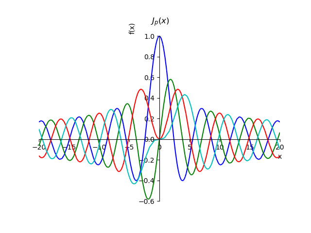
Using the relation for the sum of a series, we can prove the property of these functions for entire orders

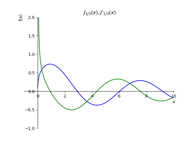
To demonstrate the Cauchy conditions, we construct a function and its derivative
  :
:
However, for practical calculations, the wonderful mpmath module is used, which allows not only numerically solving equations with Bessel functions of the first and second kind, including modified ones of all admissible orders, but also constructing graphs with automatic scaling.
In addition, the mpmath module does not require special tools for sharing symbolic and numerical mathematics. The history of the creation of this module and the possibility of its use for the inverse Laplace transform I have already considered in publication [2]. Now we continue the discussion of mpmath for working with Bessel functions [3].
Bessel function of the first kind
mpmath.besselj (n, x, derivative = 0) - gives a Bessel function of the first kind . Functions is a solution to the following differential equation:
For the whole positive behaves like a sine or cosine, multiplied by a coefficient that slowly decreases with
Bessel function of the first kind is a special case of hypergeometric function  :
:
Bessel function can be differentiated times provided that the mth derivative is not equal to zero:
Bessel function of the first kind for positive integer orders n = 0,1,2,3 - the solution of the Bessel equation:

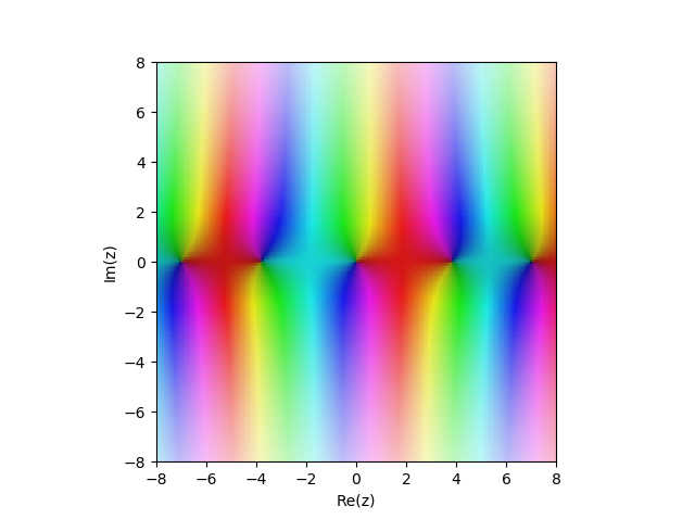
Bessel function of the first kind in the complex plane:
Examples:
Function provides a result with a given number of digits
  after comma:
A function argument can be a large number:
Bessel functions of the first kind satisfy simple symmetries with respect to :
:
The roots are not periodic, but the distance between successive roots asymptotically approaches . Bessel functions of the first kind have the following code:
For or Bessel function is reduced to a trigonometric function:
Derivatives of any order can be calculated, negative orders correspond to integration :
Differentiation with non-integer order gives a fractional derivative in the sense of the Riemann-Liouville differential integral, calculated using the function :
:
Other ways to call the Bessel function of the first kind of zero and first order
mpmath.j0 (x) - Computes the Bessel function;
mpmath.j1 (x) - Computes the Bessel function;
Bessel functions of the second kind
bessely (n, x, derivative = 0) Calculates the Bessel function of the second kind by the ratio:
For an integerThe following formula should be understood as the limit. Bessel function can be differentiated times provided that the mth derivative is not equal to zero:

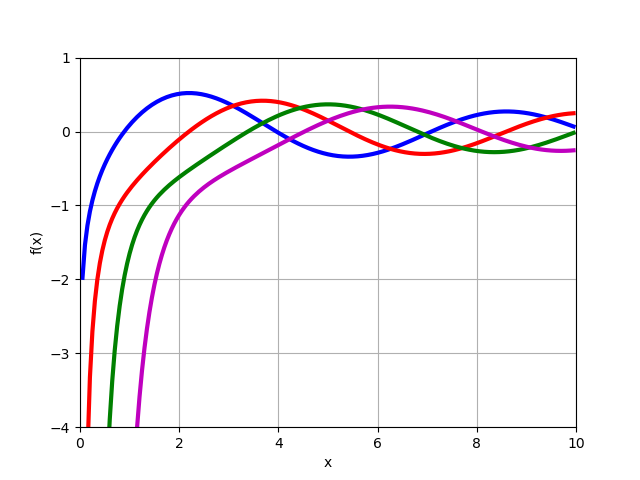
Bessel function of the second kind for integer positive orders
  .
.
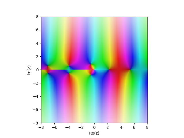
2nd kind Bessel function in the complex plane
Examples:
Some function values:
Arguments can be large:
Derivatives of any order, including negative, can be calculated:
Modified Bessel function of the first kind
besseli (n, x, derivative = 0) modified Bessel function of the first kind
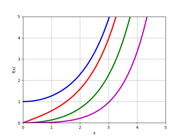
Modified Bessel Function for real orders :
Modified Bessel Function in the complex plane

Examples:
Some values
Arguments can be large:
For integers n, the following integral representation holds:
Derivatives of any order can be calculated:
Modified Bessel functions of the second kind,
besselk (n, x) modified second-kind Bessel functions
For an integerthis formula should be understood as a limit.
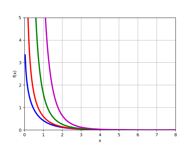
Modified Bessel function of the 2nd kind for material :
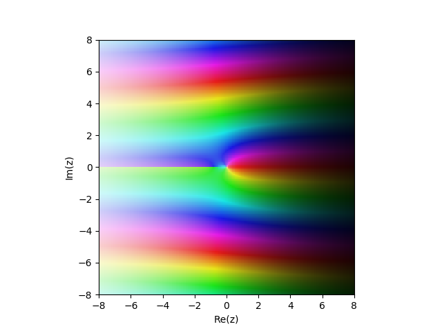
Modified Bessel function of the 2nd kind in the complex plane
Examples:
Complex and complex arguments:
Arguments are Big Numbers
Features of the behavior of a function at a point:
Bessel Function Zeros
For real order and a positive integer returns
  , the mth positive zero of the Bessel function of the first kind
  (see besselj () ). Alternatively, with
 gives the first non-negative prime zero
  of
of  . Indexing agreement designations using Abramowitz & Stegun and DLMF. Pay attention to a special case.
 while all other zeros are positive.
In reality, only simple zeros are calculated (all zeros of the Bessel functions are simple, except when ), and becomes a monotonic function of
  and . Zeros alternate according to the inequalities:
Examples:
Leading zeros of Bessel functions ,
, ,
,
Leading zeros of derivatives of Bessel functions ,
, ,
,
Zeros with a large index:
Zeros of functions with a large order:
Zeros of functions with fractional order:
AND. and can be expressed as infinite products at their zeros:
For real order and a positive integer returns  , , mth positive zero of the second kind of Bessel function
  (see Bessely () ). Alternatively, withgives the first positive zero
  of
of  . Zeros alternate according to the inequalities:
Examples:
Leading zeros of Bessel functions ,
, ,
,
Leading zeros of derivatives of Bessel functions ,
, ,
,
Zeros with a large index:
Zeros of functions with a large order:
Zeros of functions with fractional order:
Applications of Bessel functions
The importance of Bessel functions is caused not only by the frequent appearance of the Bessel equation in applications, but also by the fact that the solutions of many other second-order linear differential equations can be expressed in terms of Bessel functions. To see how they appear, we start with the Bessel equation of order in the shape of:
and substitute here
Then, using (2) and introducing the constants from equation (1), we obtain:
From equation (4) we get:
If ,
,  ,
,  , then the general solution (for
  ) of equation (3) has the form:
Where: ,
,  ,
,  are determined from system (5). If Is an integer then
  need to be replaced by
  .
.
Longitudinal bending of a vertical column
We now consider a problem that is important for practical applications. In this task, it is required to determine when a uniform vertical column is bent under its own weight. We presume in the free upper end of the column and  at its base; we assume that the base is rigidly inserted (i.e., fixed motionless) into the base (into the ground), possibly into concrete.
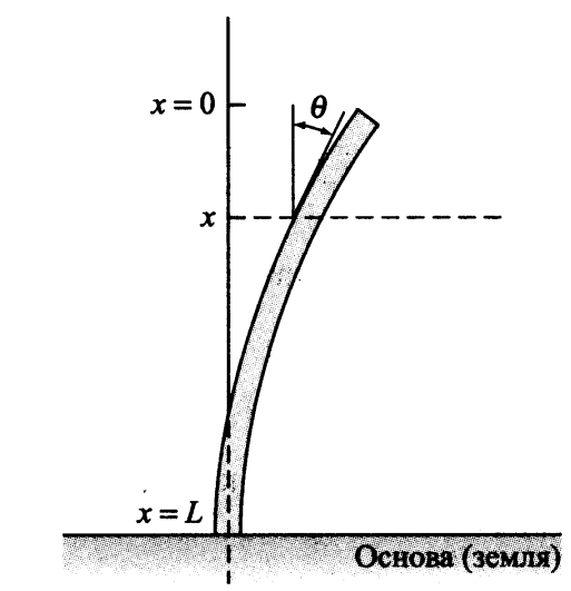
Denote the angular deviation of the column at the point through  . From the theory of elasticity under these conditions it follows that:
Where - Young's modulus of the column material,  - moment of inertia of its cross section,
  - linear density of the column and
  - gravitational acceleration. The boundary conditions are of the form:
We will solve the problem using (7) and (8) with:
We rewrite (7) taking into account (9) under condition (8):
A column can be deformed only if there is a non-trivial solution to problem (10); otherwise, the column will remain in a position not deviated from the vertical (i.e., physically unable to deviate from the vertical).
Differential equation (10) is an Airy equation. Equation (10) has the form of equation (3) for ,
,  ,
,  . From the system of equations (5) we obtain
 ,
,  ,
,  ,
,  .
.
Therefore, the general solution has the form:
To apply the initial conditions, we substitute in
in
After transformation (12), taking into account solution (11), we obtain:
Provided at the starting point we get
  , then (11) takes the form:
Provided at the end point , from (14) we get:
It should be noted that transformations (13), (14) could not be done if the graphs of functions were constructed using the considered capabilities of the mpmath module:
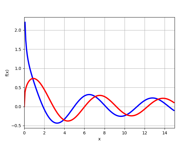
From the graph it follows that for x = 0 the function and taking into account solution (11), we immediately obtain the necessary equation (15), it remains only to find z, as will be shown below.
Thus, the column is deformed only if - root of the equation
  . Build a function
 on a separate chart:

The graph shows that the first root is slightly less than 2. Find the root from the equation You can, using the findroot (f, z0) function , accepting, according to the graph, the search point
 and six decimal places mp.dps = 6 :
We get:

We calculate the critical length, for example, a flagpole, using the formula (15):
We get:
8.47 m
10.25 m The
hollow flagpole can be higher than the solid one.
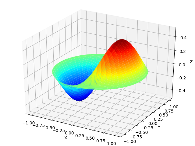
A thin membrane when sound waves enter it not only oscillates with the frequency of the waves. The form of membrane vibrations can be obtained in the Bessel functions according to the following listing, using the formulas besselj () and besseljzero () :
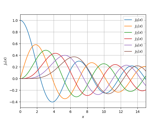
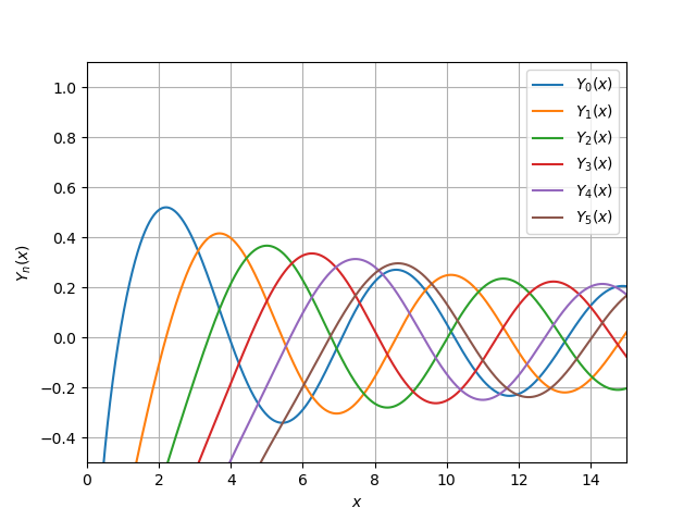
Without delving into a detailed discussion of Bessel functions from the SciPy library [4], I will give only two listings for plotting functions of the first and second kind jv (v, x) , yv (v, x) :
The article describes the basics of working with Bessel functions using the mpmath, sympy and scipy libraries, provides examples of using functions to solve differential equations. The article may be useful in studying the equations of mathematical physics.
1. Bessel functions
2. Using the inverse Laplace transform to analyze the dynamic links of control systems
3. Bessel function related functions
4. Special functions (scipy.special).
A large number of the most diverse problems related to almost all the most important branches of mathematical physics and designed to answer topical technical questions are related to the application of Bessel functions.
Bessel functions are widely used in solving problems of acoustics, radiophysics, hydrodynamics, problems of atomic and nuclear physics. Numerous applications of the Bessel functions to the theory of thermal conductivity and the theory of elasticity (problems on plate vibrations, problems of shell theory, problems of determining the stress concentration near cracks).
Such popularity of Bessel functions is explained by the fact that solving equations of mathematical physics containing the Laplace operator in cylindrical coordinates by the classical method of separation of variables leads to an ordinary differential equation, which serves to determine these functions [1].
Bessel functions are named after the German astronomer Friedrich Bessel, who in 1824, studying the motion of planets around the sun, derived recurrence relations for Bessel functions
received for integers integral representation of a function , proved the existence of countless zeros of function and compiled the first tables for functions and . However, for the first time one of the functions of Bessel
It was considered back in 1732 by Daniel Bernoulli in a work devoted to the oscillation of heavy chains. D. Bernoulli found an expression of function in the form of a power series and noticed (without proof) that the equation has countless valid roots. The next work, in which Bessel functions are encountered, was the work of Leonardo Euler in 1738, devoted to the study of vibrations of a circular membrane. In this work, L. Euler found for integers
Bessel function expression in the form of a series in powers , and in subsequent papers extended this expression to the case of arbitrary index values . In addition, L. Euler proved that forequal to an integer and a half, functions expressed through elementary functions. He noted (without evidence) that with valid
the functions have countless real zeros and gave an integral representation for . Some researchers believe that the main results related to Bessel functions and their applications in mathematical physics are connected with the name of L. Euler. To study the property of Bessel functions and at the same time to master methods for solving equations that are reduced to Bessel functions, allows the freely distributed program of symbolic mathematics SymPy - the Python library.
In the SymPy symbolic mathematics program, graphs of Bessel functions of the first kind of integer orders can be constructed using the relation for the sum of a series:

Bessel functions of the first kind
from sympy import*
from sympy.plotting import plot
x,n, p=var('x,n, p')
def besselj(p,x):
    return summation(((-1)**n*x**(2*n+p))/(factorial(n)*gamma(n+p+1)*2**(2*n+p)),[n,0,oo])
st="J_{p}(x)"
p1=plot(besselj(0,x),(x,-20,20),line_color='b',title=' $'+st+ '$',show=False)
p2=plot(besselj(1,x),(x,-20,20),line_color='g',show=False)
p3=plot(besselj(2,x),(x,-20,20),line_color='r',show=False)
p4=plot(besselj(3,x),(x,-20,20),line_color='c',show=False)
p1.extend(p2)
p1.extend(p3)
p1.extend(p4)
p1.show()
Using the relation for the sum of a series, we can prove the property of these functions for entire orders

Property of the Bessel function of the first kind
from sympy import*
from sympy.plotting import plot
x,n, p=var('x,n, p')
def besselj(p,x):
    return summation(((-1)**n*x**(2*n+p))/(factorial(n)*gamma(n+p+1)*2**(2*n+p)),[n,0,oo])
st="J_{1}(x)=-J_{-1}(x)"
p1=plot(besselj(1,x),(x,-10,10),line_color='b',title=' $'+st+ '$',show=False)
p2=plot(besselj(-1,x),(x,-10,10),line_color='r',show=False)
p1.extend(p2)
p1.show()
To demonstrate the Cauchy conditions, we construct a function
and its derivative :Fractional order function and its derivative
from sympy import*
from sympy.plotting import plot
x,n, p=var('x,n, p')
def besselj(p,x):
    return summation(((-1)**n*x**(2*n+p))/(factorial(n)*gamma(n+p+1)*2**(2*n+p)),[n,0,oo])
st="J_{1/3}(x),J{}'_{1/3}(x)"
p1=plot(besselj(1/3,x),(x,-1,10),line_color='b',title=' $'+st+ '$',ylim=(-1,2),show=False)
def dbesselj(p,x):
    return diff(summation(((-1)**n*x**(2*n+p))/(factorial(n)*gamma(n+p+1)*2**(2*n+p)),[n,0,oo]),x)
p2=plot(dbesselj(1/3,x),(x,-1,10),line_color='g',show=False)
p1.extend(p2)
p1.show()
However, for practical calculations, the wonderful mpmath module is used, which allows not only numerically solving equations with Bessel functions of the first and second kind, including modified ones of all admissible orders, but also constructing graphs with automatic scaling.
In addition, the mpmath module does not require special tools for sharing symbolic and numerical mathematics. The history of the creation of this module and the possibility of its use for the inverse Laplace transform I have already considered in publication [2]. Now we continue the discussion of mpmath for working with Bessel functions [3].
Bessel function of the first kind
mpmath.besselj (n, x, derivative = 0) - gives a Bessel function of the first kind
. Functions is a solution to the following differential equation:
For the whole positive
behaves like a sine or cosine, multiplied by a coefficient that slowly decreases with Bessel function of the first kind
is a special case of hypergeometric function :
Bessel function can be differentiated
times provided that the mth derivative is not equal to zero:
Bessel function of the first kind
for positive integer orders n = 0,1,2,3 - the solution of the Bessel equation:
from mpmath import*
j0 = lambda x: besselj(0,x)
j1 = lambda x: besselj(1,x)
j2 = lambda x: besselj(2,x)
j3 = lambda x: besselj(3,x)
plot([j0,j1,j2,j3],[0,14]
Bessel function of the first kind
in the complex plane:from sympy import*
from mpmath import*
cplot(lambda z: besselj(1,z), [-8,8], [-8,8], points=50000)Examples:
Function
provides a result with a given number of digits after comma:
from mpmath import*
mp.dps = 15; mp.pretty = True
print(besselj(2, 1000))
nprint(besselj(4, 0.75))
nprint(besselj(2, 1000j))
mp.dps = 25
nprint( besselj(0.75j, 3+4j))
mp.dps = 50
nprint( besselj(1, pi))
A function argument can be a large number:
from mpmath import*
mp.dps = 25
nprint( besselj(0, 10000))
nprint(besselj(0, 10**10))
nprint(besselj(2, 10**100))
nprint( besselj(2, 10**5*j))
Bessel functions of the first kind satisfy simple symmetries with respect to
:from sympy import*
from mpmath import*
mp.dps = 15
nprint([besselj(n,0) for n in range(5)])
nprint([besselj(n,pi) for n in range(5)])
nprint([besselj(n,-pi) for n in range(5)])The roots are not periodic, but the distance between successive roots asymptotically approaches
. Bessel functions of the first kind have the following code:
from mpmath import*
print(quadosc(j0, [0, inf], period=2*pi))
print(quadosc(j1, [0, inf], period=2*pi))
For
or Bessel function is reduced to a trigonometric function:from sympy import*
from mpmath import*
x = 10
print(besselj(0.5, x))
print(sqrt(2/(pi*x))*sin(x))
print(besselj(-0.5, x))
print(sqrt(2/(pi*x))*cos(x))Derivatives of any order can be calculated, negative orders correspond to integration :
from mpmath import*
mp.dps = 25
print(besselj(0, 7.5, 1))
print(diff(lambda x: besselj(0,x), 7.5))
print(besselj(0, 7.5, 10))
print(diff(lambda x: besselj(0,x), 7.5, 10))
print(besselj(0,7.5,-1) - besselj(0,3.5,-1))
print(quad(j0, [3.5, 7.5]))
Differentiation with non-integer order gives a fractional derivative in the sense of the Riemann-Liouville differential integral, calculated using the function
:
from mpmath import*
mp.dps = 15
print(besselj(1, 3.5, 0.75))
print(differint(lambda x: besselj(1, x), 3.5, 0.75))
Other ways to call the Bessel function of the first kind of zero and first order
mpmath.j0 (x) - Computes the Bessel function
; mpmath.j1 (x) - Computes the Bessel function
; Bessel functions of the second kind
bessely (n, x, derivative = 0) Calculates the Bessel function of the second kind by the ratio:

For an integer
The following formula should be understood as the limit. Bessel function can be differentiated times provided that the mth derivative is not equal to zero:Bessel function of the second kind
for integer positive orders .from sympy import*
from mpmath import*
y0 = lambda x: bessely(0,x)
y1 = lambda x: bessely(1,x)
y2 = lambda x: bessely(2,x)
y3 = lambda x: bessely(3,x)
plot([y0,y1,y2,y3],[0,10],[-4,1])2nd kind Bessel function
in the complex planefrom sympy import*
from mpmath import*
cplot(lambda z: bessely(1,z), [-8,8], [-8,8], points=50000)Examples:
Some function values
:from sympy import*
from mpmath import*
mp.dps = 25; mp.pretty = True
print(bessely(0,0))
print(bessely(1,0))
print(bessely(2,0))
print(bessely(1, pi))
print(bessely(0.5, 3+4j))Arguments can be large:
from sympy import*
from mpmath import*
mp.dps = 25; mp.pretty = True
print(bessely(0, 10000))
print(bessely(2.5, 10**50))
print(bessely(2.5, -10**50))
Derivatives of any order, including negative, can be calculated:
from sympy import*
from mpmath import*
mp.dps = 25; mp.pretty = True
print(bessely(2, 3.5, 1))
print(diff(lambda x: bessely(2, x), 3.5))
print(bessely(0.5, 3.5, 1))
print(diff(lambda x: bessely(0.5, x), 3.5))
print(diff(lambda x: bessely(2, x), 0.5, 10))
print(bessely(2, 0.5, 10))
print(bessely(2, 100.5, 100))
print(quad(lambda x: bessely(2,x), [1,3]))
print(bessely(2,3,-1) - bessely(2,1,-1))
Modified Bessel function of the first kind
mpmath.besseli(n, x, derivative=0)besseli (n, x, derivative = 0) modified Bessel function of the first kind


Modified Bessel Function
for real orders :from mpmath import*
i0 = lambda x: besseli(0,x)
i1 = lambda x: besseli(1,x)
i2 = lambda x: besseli(2,x)
i3 = lambda x: besseli(3,x)
plot([i0,i1,i2,i3],[0,5],[0,5])Modified Bessel Function
in the complex planefrom mpmath import*
cplot(lambda z: besseli(1,z), [-8,8], [-8,8], points=50000)Examples:
Some values
from mpmath import*
mp.dps = 25; mp.pretty = True
print(besseli(0,0))
print(besseli(1,0))
print(besseli(0,1))
print(besseli(3.5, 2+3j))
Arguments can be large:
from mpmath import*
mp.dps = 25; mp.pretty = True
print(besseli(2, 1000))
print(besseli(2, 10**10))
print(besseli(2, 6000+10000j))
For integers n, the following integral representation holds:
from mpmath import*
mp.dps = 15; mp.pretty = True
n = 3
x = 2.3
print(quad(lambda t: exp(x*cos(t))*cos(n*t), [0,pi])/pi)
print(besseli(n,x))
Derivatives of any order can be calculated:
from mpmath import*
mp.dps = 25; mp.pretty = True
print(besseli(2, 7.5, 1))
print(diff(lambda x: besseli(2,x), 7.5))
print(besseli(2, 7.5, 10))
print(diff(lambda x: besseli(2,x), 7.5, 10))
print(besseli(2,7.5,-1) - besseli(2,3.5,-1))
print(quad(lambda x: besseli(2,x), [3.5, 7.5]))
Modified Bessel functions of the second kind,
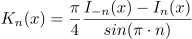
mpmath.besselk(n, x)besselk (n, x) modified second-kind Bessel functions
For an integer
this formula should be understood as a limit. Modified Bessel function of the 2nd kind
for material :from mpmath import*
k0 = lambda x: besselk(0,x)
k1 = lambda x: besselk(1,x)
k2 = lambda x: besselk(2,x)
k3 = lambda x: besselk(3,x)
plot([k0,k1,k2,k3],[0,8],[0,5])Modified Bessel function of the 2nd kind
in the complex planefrom mpmath import*
cplot(lambda z: besselk(1,z), [-8,8], [-8,8], points=50000)Examples:
Complex and complex arguments:
from mpmath import *
mp.dps = 25; mp.pretty = True
print(besselk(0,1))
print(besselk(0, -1))
print(besselk(3.5, 2+3j))
print(besselk(2+3j, 0.5))
Arguments are Big Numbers
from mpmath import *
mp.dps = 25; mp.pretty = True
print(besselk(0, 100))
print(besselk(1, 10**6))
print(besselk(1, 10**6*j))
print(besselk(4.5, fmul(10**50, j, exact=True)))
Features of the behavior of a function at a point
:from mpmath import *
print(besselk(0,0))
print(besselk(1,0))
for n in range(-4, 5):
print(besselk(n, '1e-1000'))Bessel Function Zeros
besseljzero()
mpmath.besseljzero(v, m, derivative=0)
For real order
and a positive integer returns , the mth positive zero of the Bessel function of the first kind (see besselj () ). Alternatively, withgives the first non-negative prime zero of . Indexing agreement designations using Abramowitz & Stegun and DLMF. Pay attention to a special case.while all other zeros are positive. In reality, only simple zeros are calculated (all zeros of the Bessel functions are simple, except when
), and becomes a monotonic function of and . Zeros alternate according to the inequalities:

Examples:
Leading zeros of Bessel functions
,,from mpmath import *
mp.dps = 25; mp.pretty = True
print(besseljzero(0,1))
print(besseljzero(0,2))
print(besseljzero(0,3))
print(besseljzero(1,1))
print(besseljzero(1,2))
print(besseljzero(1,3))
print(besseljzero(2,1))
print(besseljzero(2,2))
print(besseljzero(2,3))Leading zeros of derivatives of Bessel functions
,,from mpmath import *
mp.dps = 25; mp.pretty = True
print(besseljzero(0,1,1))
print(besseljzero(0,2,1))
print(besseljzero(0,3,1))
print(besseljzero(1,1,1))
print(besseljzero(1,2,1))
print(besseljzero(1,3,1))
print(besseljzero(2,1,1))
print(besseljzero(2,2,1))
print(besseljzero(2,3,1))Zeros with a large index:
from mpmath import *
mp.dps = 25; mp.pretty = True
print(besseljzero(0,100))
print(besseljzero(0,1000))
print(besseljzero(0,10000))
print(besseljzero(5,100))
print(besseljzero(5,1000))
print(besseljzero(5,10000))
print(besseljzero(0,100,1))
print(besseljzero(0,1000,1))
print(besseljzero(0,10000,1))
Zeros of functions with a large order:
from mpmath import *
mp.dps = 25; mp.pretty = True
print(besseljzero(50,1))
print(besseljzero(50,2))
print(besseljzero(50,100))
print(besseljzero(50,1,1))
print(besseljzero(50,2,1))
print(besseljzero(50,100,1))
Zeros of functions with fractional order:
from mpmath import *
mp.dps = 25; mp.pretty = True
print(besseljzero(0.5,1))
print(besseljzero(1.5,1))
print(besseljzero(2.25,4))
AND
. and can be expressed as infinite products at their zeros:from mpmath import *
mp.dps = 6; mp.pretty = True
v,z = 2, mpf(1)
nprint((z/2)**v/gamma(v+1) * \
nprod(lambda k: 1-(z/besseljzero(v,k))**2, [1,inf]))
print(besselj(v,z))
nprint((z/2)**(v-1)/2/gamma(v) * \
nprod(lambda k: 1-(z/besseljzero(v,k,1))**2, [1,inf]))
print(besselj(v,z,1))besselyzero()
mpmath.besselyzero(v, m, derivative=0)For real order
and a positive integer returns , , mth positive zero of the second kind of Bessel function (see Bessely () ). Alternatively, withgives the first positive zero of . Zeros alternate according to the inequalities:

Examples:
Leading zeros of Bessel functions
,,from mpmath import *
mp.dps = 25; mp.pretty = True
print(besselyzero(0,1))
print(besselyzero(0,2))
print(besselyzero(0,3))
print(besselyzero(1,1))
print(besselyzero(1,2))
print(besselyzero(1,3))
print(besselyzero(2,1))
print(besselyzero(2,2))
print(besselyzero(2,3))Leading zeros of derivatives of Bessel functions
,,from mpmath import *
mp.dps = 25; mp.pretty = True
print(besselyzero(0,1,1))
print(besselyzero(0,2,1))
print(besselyzero(0,3,1))
print(besselyzero(1,1,1))
print(besselyzero(1,2,1))
print(besselyzero(1,3,1))
print(besselyzero(2,1,1))
print(besselyzero(2,2,1))
print(besselyzero(2,3,1))Zeros with a large index:
from mpmath import *
mp.dps = 25; mp.pretty = True
print(besselyzero(0,100))
print(besselyzero(0,1000))
print(besselyzero(0,10000))
print(besselyzero(5,100))
print(besselyzero(5,1000))
print(besselyzero(5,10000))
print(besselyzero(0,100,1))
print(besselyzero(0,1000,1))
print(besselyzero(0,10000,1))
Zeros of functions with a large order:
from mpmath import *
mp.dps = 25; mp.pretty = True
print(besselyzero(50,1))
print(besselyzero(50,2))
print(besselyzero(50,100))
print(besselyzero(50,1,1))
print(besselyzero(50,2,1))
print(besselyzero(50,100,1))
Zeros of functions with fractional order:
from mpmath import *
mp.dps = 25; mp.pretty = True
print(besselyzero(0.5,1))
print(besselyzero(1.5,1))
print(besselyzero(2.25,4))
Applications of Bessel functions
The importance of Bessel functions is caused not only by the frequent appearance of the Bessel equation in applications, but also by the fact that the solutions of many other second-order linear differential equations can be expressed in terms of Bessel functions. To see how they appear, we start with the Bessel equation of order
in the shape of:
and substitute here

Then, using (2) and introducing the constants
from equation (1), we obtain:

From equation (4) we get:
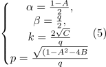
If
, , , then the general solution (for ) of equation (3) has the form:![$y(x)=x^{\alpha}\left [c_{1}J_{p}(kx^{\beta})+c_{2}J_{-p}(kx^{\beta })\right] (6)$](https://habrastorage.org/getpro/habr/formulas/990/5b8/57f/9905b857f1baf38d852b746f29dd6555.svg)
Where:
, , are determined from system (5). If Is an integer then need to be replaced by . Longitudinal bending of a vertical column
We now consider a problem that is important for practical applications. In this task, it is required to determine when a uniform vertical column is bent under its own weight. We presume
in the free upper end of the column and at its base; we assume that the base is rigidly inserted (i.e., fixed motionless) into the base (into the ground), possibly into concrete. Denote the angular deviation of the column at the point
through . From the theory of elasticity under these conditions it follows that: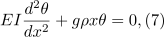
Where
- Young's modulus of the column material, - moment of inertia of its cross section, - linear density of the column and - gravitational acceleration. The boundary conditions are of the form:
We will solve the problem using (7) and (8) with:
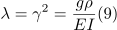
We rewrite (7) taking into account (9) under condition (8):

A column can be deformed only if there is a non-trivial solution to problem (10); otherwise, the column will remain in a position not deviated from the vertical (i.e., physically unable to deviate from the vertical).
Differential equation (10) is an Airy equation. Equation (10) has the form of equation (3) for
, , . From the system of equations (5) we obtain, , , . Therefore, the general solution has the form:
![$\theta(x)=x^{1/2}\left [c_{1}J_{1/3}(\frac{2}{3}\gamma x^{3/2})+c_{2}J_{-1/3}(\frac{2}{3}\gamma x^{3/2})\right ]. (11)$](https://habrastorage.org/getpro/habr/formulas/0da/07f/b4d/0da07fb4dec88667f0bb9ea3cbfef9a7.svg)
To apply the initial conditions, we substitute
in
After transformation (12), taking into account solution (11), we obtain:

Provided at the starting point
we get , then (11) takes the form:
Provided at the end point
, from (14) we get: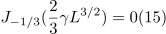
It should be noted that transformations (13), (14) could not be done if the graphs of functions were constructed
using the considered capabilities of the mpmath module:from mpmath import*
mp.dps = 6; mp.pretty = True
f=lambda x: besselj(-1/3,x)
f1=lambda x: besselj(1/3,x)
plot([f,f1], [0, 15])From the graph it follows that for x = 0 the function
and taking into account solution (11), we immediately obtain the necessary equation (15), it remains only to find z, as will be shown below. Thus, the column is deformed only if
- root of the equation . Build a function on a separate chart:from mpmath import*
mp.dps = 6; mp.pretty = True
f=lambda x: besselj(-1/3,x)
plot(f, [0, 15])The graph shows that the first root is slightly less than 2. Find the root
from the equation You can, using the findroot (f, z0) function , accepting, according to the graph, the search pointand six decimal places mp.dps = 6 :from mpmath import*
mp.dps = 6; mp.pretty = True
f=lambda x: besselj(-1/3,x)
print("z0=%s"%findroot(f, 1)We get:
We calculate the critical length, for example, a flagpole, using the formula (15):
Flagpole height for different parameters in section
from numpy import*
def LRr(R,r):
    E=2.9*10**11#н/м^2
    rou=7900#кг/м^3
    g=9.8#м/с^2
    I=pi*((R-r)**4)/4#м^4
    F=pi*(R-r)**2#м^2
    return 1.086*(E*I/(rou*g*F))**1/3
R=5*10**-3
r=0
L= LRr(R,r)
print(round(L,2),"м")
R=7.5*10**-3
r=2*10**-3
Lr= LRr(R,r)
print(round(Lr,2),"м")
We get:
8.47 m
10.25 m The
hollow flagpole can be higher than the solid one.
Wave propagation in a thin membrane.
A thin membrane when sound waves enter it not only oscillates with the frequency of the waves. The form of membrane vibrations can be obtained in the Bessel functions according to the following listing, using the formulas besselj () and besseljzero () :
Membrane Waveform
from mpmath import*
from numpy import*
import matplotlib.pyplot as plt
from mpl_toolkits.mplot3d import Axes3D
from matplotlib import cm
def Membrana(r):
    mp.dps=25
    return cos(0.5) * cos( theta) *float(besselj(1,r*besseljzero(1,1) ,0))
theta =linspace(0,2*pi,50)
radius = linspace(0,1,50)
x = array([r * cos(theta) for r in radius])
y = array([r * sin(theta) for r in radius])
z = array([Membrana(r) for r in radius])
fig = plt.figure("Мембрана")
ax = Axes3D(fig)
ax.plot_surface(x, y, z, rstride=1, cstride=1, cmap=cm.jet)
ax.set_xlabel('X')
ax.set_ylabel('Y')
ax.set_zlabel('Z')
plt.show()
Alternative to mpmath module in special Bessel functions of SciPy library
Without delving into a detailed discussion of Bessel functions from the SciPy library [4], I will give only two listings for plotting functions of the first and second kind jv (v, x) , yv (v, x) :
jv (v, x)
import numpy as np
import pylab as py
import scipy.special as sp
x = np.linspace(0, 15, 500000)
for v in range(0, 6):
    py.plot(x, sp.jv(v, x))
py.xlim((0, 15))
py.ylim((-0.5, 1.1))
py.legend(('$J_{0}(x)$', '$ J_{1}(x)$', '$J_{2}(x)$',
           '$J_{3}(x)$', '$ J_{4}(x)$','$ J_{5}(x)$'),
           loc = 0)
py.xlabel('$x$')
py.ylabel('${J}_n(x)$')
py.grid(True)
py.show()
yv (v, x)
import numpy as np
import pylab as py
import scipy.special as sp
x = np.linspace(0, 15, 500000)
for v in range(0, 6):
    py.plot(x, sp.yv(v, x))
py.xlim((0, 15))
py.ylim((-0.5, 1.1))
py.legend(('$Y_{0}(x)$', '$ Y_{1}(x)$', '$Y_{2}(x)$',
           '$Y_{3}(x)$', '$ Y_{4}(x)$','$ Y_{5}(x)$'),
           loc = 0)
py.xlabel('$x$')
py.ylabel('$Y_{n}(x)$')
py.grid(True)
py.show()
Conclusions:
The article describes the basics of working with Bessel functions using the mpmath, sympy and scipy libraries, provides examples of using functions to solve differential equations. The article may be useful in studying the equations of mathematical physics.
References:
1. Bessel functions
2. Using the inverse Laplace transform to analyze the dynamic links of control systems
3. Bessel function related functions
4. Special functions (scipy.special).