Tasks from school textbook II
Part I
Part II
This article discusses the method of evaluating the range of accepted values and the relationship of this method with tasks containing the module.
When solving some problems, it is necessary to consider the range within which the desired value can be.
Consider the estimation method for solving inequalities.
Suppose that the price per unit of goods can range from 5 to 10 RUB. To give an upper bound means to determine the maximum value that the desired quantity can take. For two units of goods, the price for which does not exceed 10, the upper estimate will be 10 + 10 = 20 .
Consider the problem fromtask book of profile orientation M.I. Bashmakova
37. Known estimates for variables and
and 
Give top marks for the following expressions:
1.
2.
5.
6.
8.
9.
In general, the analysis of infinitesimal quantities uses an evaluation criterion. The concept of a module as a neighborhood lies in the very definition of the limit.
Consider the example from the "Course of differential and integral calculus" 363 (6)
 really more
  , you need to make a lower estimate of this expression. We obtain the system of inequalities
After adding all the inequalities of this system, we get
This is proof that this series diverges.
With a harmonic range, this technique does not work, because partial harmonic series
We return to task
38. Calculate the amount ("Tasks for children from 5 to 15 years old")
(with an error of not more than 1% of the answer)
An upper estimate of the sum of the series gives the number 1.
Drop the first term
Get
0.41666666666666663
0.49019607843137253
0.4990019960079833
0.4999000199960005
0.49999000019998724
0.4999990000019941
You can check in ideone.com here
Drop the first two terms
We get 0.33333233333632745. The
partial sums of the series are bounded above.
Throw awayinitial terms of the harmonic series.
Prove (using the lower bound) that
We calculate the partial amounts that are obtained by discarding terms.
We
get : 0.5833333333333334
0.6345238095238095
0.6628718503718504
Let's write a program that calculates the sum of the harmonic series from before where
  at
at 
We
get : 0.583333333333333333
0.6345238095238095
0.6628718503718504
0.6777662022075267
You can check in online ide at the link
For range![$ \ left [1 + 2 ^ {70}; 2 ^ {71} \ right] $](https://habrastorage.org/getpro/habr/formulas/399/9b7/a38/3999b7a38c228e220ad033835860806a.svg) we get 0.693147 ...
we get 0.693147 ...
Check modzhno in Wolfram Cloud here .
This recursive algorithm causes a fast stack overflow.
In this article there is an example of the factorial using an iterative algorithm. We modify this iterative algorithm so that it calculates the partial sum Hn within certain boundaries; call these boundaries a and b
The lower bound is the number , the upper bound is the number
We write a function that calculates the power of two
We will substitute (+ 1 (power_of_two k)) as the lower boundary, and use the function (* 2 (power_of_two k)) or its equivalent function (power_of_two (+ 1 k)) as the upper boundary. Rewrite the
function Hn
Now you can calculate Hn for large values .
.
We write in C a program that measures the time required to calculate Hn . We will use the clock () function from the standard library
An article about measuring processor time is on Habré here .
Обычно online ide ограничивают время выполнения запускаемых программ пятью секундами, поэтому эту программу можно проверить лишь в некоторых online ide, например, в onlinegdb.com или repl.it
При k от 1+2^30 до 2^31 время работы составит ~5 сек.
При k от 1+2^31 до 2^32 время работы составит ~10 сек.
При k от 1+2^32 до 2^33 время работы составит ~20 сек.
При k от 1+2^33 до 2^34 время работы составит ~40 сек.
При k от 1+2^34 до 2^35 время работы составит больше одной минуты.
…
При k от 1+2^45 до 2^46 время работы составит больше 24 часов.
Предположим, что для k от 1+2^30 до 2^31 время выполнения алгоритма составляет ~2 сек.
Тогда для k=2^(30+n) время выполнения алгоритма составляет 2^n сек. (при )
)
Данный алгоритм имеет экспотенциальную сложность.
Вернёмся к модулям.
В интегральном исчислении модуль используется в формуле
На Хабре была статья Самый натуральный логарифм, в которой рассматривается этот интеграл и на основе его вычисление числа .
.
Присутствие модуля в формуле обосновывается далее в «Курсе дифференциального и интегрального исчисления»
Физическое приложение интеграла
Этот интеграл используется для вычисления разности потенциалов обкладок цилиндрического конденсатора.

«Электричество и магнетизм»:
 , because
  and
and  strictly positive and this form of recording is redundant.
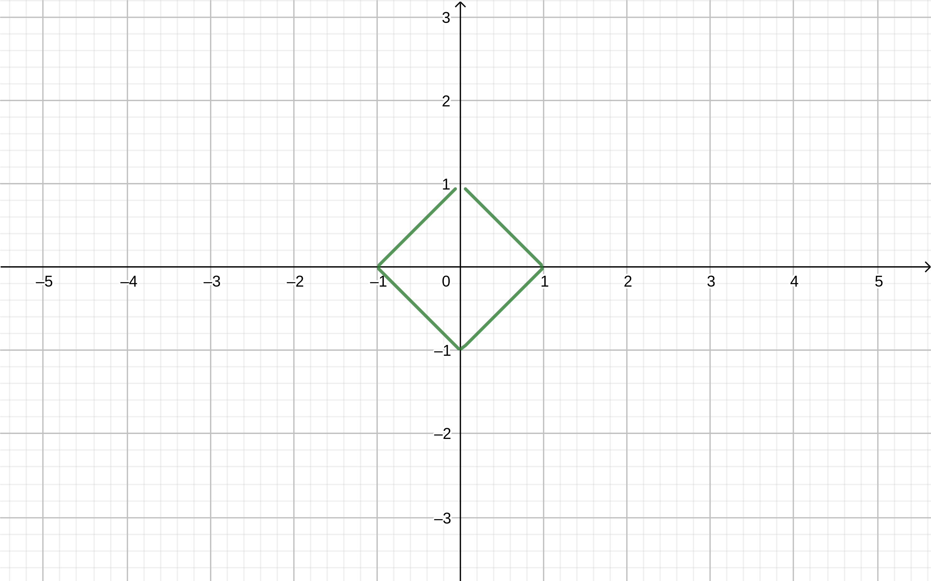
Using modules, you can draw various shapes.
If in the geogebra program write the formula get.
get.
You can draw more complex shapes. Let's draw, for example, a “butterfly” in the WolframAlpha cloud
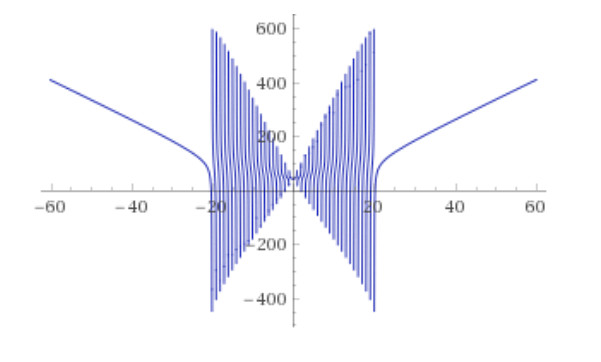
Plot [Sum [abs (x) / (n-abs (x)) + abs (x + n) / (n) + abs (xn) / (n), {n, 1,20}], {x, -60.60}]
In this expression lies in the range from  before
  , lies in the range from
  before
  .
.
Link to the picture.
“The task book of profile orientation” M.I. Bashmakov
General physics course: in 3 volumes T. 2. “Electricity and magnetism” I.V. Savelyev
Part II
This article discusses the method of evaluating the range of accepted values and the relationship of this method with tasks containing the module.
When solving some problems, it is necessary to consider the range within which the desired value can be.
Consider the estimation method for solving inequalities.
Suppose that the price per unit of goods can range from 5 to 10 RUB. To give an upper bound means to determine the maximum value that the desired quantity can take. For two units of goods, the price for which does not exceed 10, the upper estimate will be 10 + 10 = 20 .
Consider the problem fromtask book of profile orientation M.I. Bashmakova
37. Known estimates for variables
and Give top marks for the following expressions:
1.
2.
Guide to solving problems 5 and 6
To evaluate fractional expressions, it is necessary to use the following property of numerical inequalities:
- If
 and both numbers are positive, then
5.
6.
Instructions for solving problems 8 and 9
To evaluate negative values, it is necessary to use the following property of numerical inequalities:
If and both numbers are positive, then 
If
and both numbers are positive, then 8.
9.
In general, the analysis of infinitesimal quantities uses an evaluation criterion. The concept of a module as a neighborhood lies in the very definition of the limit.

Consider the example from the "Course of differential and integral calculus" 363 (6)
Easy to set row divergenceIn order to prove that
In fact, since its members decrease, the nth partial sum
and grows ad infinitum with

 really more , you need to make a lower estimate of this expression. We obtain the system of inequalities
After adding all the inequalities of this system, we get

This is proof that this series diverges.
With a harmonic range, this technique does not work, because
partial harmonic series 
We return to task
38. Calculate the amount ("Tasks for children from 5 to 15 years old")

(with an error of not more than 1% of the answer)
An upper estimate of the sum of the series
gives the number 1. Drop the first term
(define series_sum_1
 ( lambda (n)
  (if (= n 0) 0
    (+ (/ 1.0 (* (+ n 1.0 )(+ n 2.0))) (series_sum_1(- n 1.0)))
  ) ) )
(writeln (series_sum_1 10))
(writeln (series_sum_1 100))
(writeln (series_sum_1 1000))
(writeln (series_sum_1 10000))
(writeln (series_sum_1 100000))
(writeln (series_sum_1 1000000))
Get
0.41666666666666663
0.49019607843137253
0.4990019960079833
0.4999000199960005
0.49999000019998724
0.4999990000019941
You can check in ideone.com here
The same algorithm in Python
Link to ideone.com
def series_sum(n):
	if n==0:
		return 0
	else:
		return 1.0/((n+1.0)*(n+2.0))+series_sum(n-1.0)
print(series_sum(10))
print(series_sum(100))
Link to ideone.com
Drop the first two terms
(define series_sum_1
 ( lambda (n)
  (if (= n 0) 0
    (+ (/ 1.0 (* (+ n 2.0) (+ n 3.0))) (series_sum_1(- n 1.0)))
  ) ) )
(series_sum_1 1000000)
We get 0.33333233333632745. The
partial sums of the series are bounded above.
The positive row always has an amount; this sum will be finite (and therefore the series converging) if the partial sums of the series are bounded above, and infinite (and the series diverging) otherwise.
We calculate the sum of the harmonic series with increasing n
We
get : 2.9289682539682538
5.187377517639621
7.485470860550343
9.787606036044348
12.090146129863335
14.392726722864989
#lang racket
(define series_sum_1
 ( lambda (n)
  (if (= n 0) 0
    (+ (/ 1.0 n) (series_sum_1(- n 1.0)))
  ) ) )
(series_sum_1 10)
(series_sum_1 100)
(series_sum_1 1000)
(series_sum_1 10000)
(series_sum_1 100000)
(series_sum_1 1000000)
We
get : 2.9289682539682538
5.187377517639621
7.485470860550343
9.787606036044348
12.090146129863335
14.392726722864989
Throw away
initial terms of the harmonic series. Prove (using the lower bound) that

If, discarding the first two terms, the remaining members of the harmonic series are divided into groups bymembers in each
then each of these amounts individually will be larger.
... We see that partial sums cannot be bounded above: the series has an infinite sum.


We calculate the partial amounts that are obtained by discarding
terms.#lang racket
(* 1.0 (+ 1/3 1/4))
(* 1.0 (+ 1/5 1/6 1/7 1/8))
(* 1.0 (+ 1/9 1/10 1/11 1/12 1/13 1/14 1/15 1/16))
We
get : 0.5833333333333334
0.6345238095238095
0.6628718503718504
Let's write a program that calculates the sum of the harmonic series from
before where at #lang racket
(define (Hn n )
(define half_arg (/ n 2.0))
(define (series_sum n)
(if (= n half_arg ) 0
(+ (/ 1.0 n) (series_sum(- n 1)) )
)
)
(series_sum n) )
(Hn 4)
(Hn 8)
(Hn 16)
(Hn 32)
We
get : 0.583333333333333333
0.6345238095238095
0.6628718503718504
0.6777662022075267
You can check in online ide at the link
For range
we get 0.693147 ... Check modzhno in Wolfram Cloud here .
This recursive algorithm causes a fast stack overflow.
In this article there is an example of the factorial using an iterative algorithm. We modify this iterative algorithm so that it calculates the partial sum Hn within certain boundaries; call these boundaries a and b
(define (Hn a b)
  (define (iteration product counter)
    (if (> counter b)
        product
        (iteration (+ product (/ 1.0 counter))
                   (+ counter 1))))
  (iteration 0 a))
The lower bound is the number
, the upper bound is the number We write a function that calculates the power of two
(define (power_of_two k)
  (define (iteration product counter)
    (if (> counter k)
        product
        (iteration (* product 2)
                   (+ counter 1))))
  (iteration 1 1))
We will substitute (+ 1 (power_of_two k)) as the lower boundary, and use the function (* 2 (power_of_two k)) or its equivalent function (power_of_two (+ 1 k)) as the upper boundary. Rewrite the
function Hn
(define (Hn k)
  (define a (+ 1 (power_of_two k)) )
  (define b (* 2 (power_of_two k)) )
  (define (iteration product counter)
    (if (> counter b)
        product
        (iteration (+ product (/ 1.0 counter))
                   (+ counter 1))))
  (iteration 0 a ))
Now you can calculate Hn for large values
. We write in C a program that measures the time required to calculate Hn . We will use the clock () function from the standard library
An article about measuring processor time is on Habré here .
#include
#include
#include
int main(int argc, char **argv)
{
double count;
// k от 1+2^30 до 2^31
for(unsigned long long int i=1073741825  ;i<=2147483648 ;i++)
{
	count=count+1.0/i;
		}
printf("Hn = %.12f ", count);
 double seconds = clock() / (double) CLOCKS_PER_SEC;
 printf("Программа работала %f сек \n", seconds);
 return 0;
}
Обычно online ide ограничивают время выполнения запускаемых программ пятью секундами, поэтому эту программу можно проверить лишь в некоторых online ide, например, в onlinegdb.com или repl.it
При k от 1+2^30 до 2^31 время работы составит ~5 сек.
При k от 1+2^31 до 2^32 время работы составит ~10 сек.
При k от 1+2^32 до 2^33 время работы составит ~20 сек.
При k от 1+2^33 до 2^34 время работы составит ~40 сек.
При k от 1+2^34 до 2^35 время работы составит больше одной минуты.
…
При k от 1+2^45 до 2^46 время работы составит больше 24 часов.
Предположим, что для k от 1+2^30 до 2^31 время выполнения алгоритма составляет ~2 сек.
Тогда для k=2^(30+n) время выполнения алгоритма составляет 2^n сек. (при
)Данный алгоритм имеет экспотенциальную сложность.
Вернёмся к модулям.
В интегральном исчислении модуль используется в формуле

На Хабре была статья Самый натуральный логарифм, в которой рассматривается этот интеграл и на основе его вычисление числа
. Присутствие модуля в формуле
обосновывается далее в «Курсе дифференциального и интегрального исчисления»Если…, то дифференцированием легко убедиться в том, что
![$ \ left [ln (-x) \ right] '= \ frac {1} {x} $](https://habrastorage.org/getpro/habr/formulas/e97/a65/809/e97a65809fdf718fd5fdd8e8f34e2b20.svg)
Физическое приложение интеграла 
Этот интеграл используется для вычисления разности потенциалов обкладок цилиндрического конденсатора.
«Электричество и магнетизм»:
Разность потенциалов между обкладками находим путем интегрирования:The module sign is not used here under the sign of the natural logarithm
(
 , because and strictly positive and this form of recording is redundant.
"Modular" drawing
Using modules, you can draw various shapes.
If in the geogebra program write the formula
get. You can draw more complex shapes. Let's draw, for example, a “butterfly” in the WolframAlpha cloud

Plot [Sum [abs (x) / (n-abs (x)) + abs (x + n) / (n) + abs (xn) / (n), {n, 1,20}], {x, -60.60}]
In this expression
lies in the range from before , lies in the range from before . Link to the picture.
Books:
“The task book of profile orientation” M.I. Bashmakov
General physics course: in 3 volumes T. 2. “Electricity and magnetism” I.V. Savelyev