iphysic March 4, 2019 at 14:02

Introducing Neural ODE

Neural Ordinary Differential Equations

A significant proportion of processes is described by differential equations, this may be the evolution of a physical system over time, the patient’s medical condition, fundamental characteristics of the stock market, etc. The data on such processes are consistent and continuous in nature, in the sense that observations are simply manifestations of some kind of continuously changing state.

There is also another type of serial data, it is discrete data, for example, NLP task data. The state in such data varies discretely: from one character or word to another.

Now both types of such serial data are usually processed by recursive networks, although they are different in nature and seem to require different approaches.

At the last NIPS conferenceOne very interesting article was presented that could help solve this problem. The authors propose an approach that they called Neural ODEs .

Here I tried to reproduce and summarize the results of this article in order to make acquaintance with her idea a little easier. It seems to me that this new architecture may well find a place in the standard tools of a data scientist along with convolutional and recurrent networks.

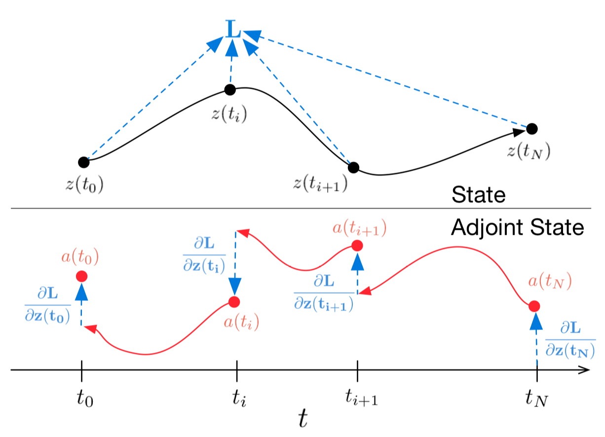
Figure 1: Continuous gradient backpropagation requires solving the augmented differential equation back in time.

The arrows represent the adjustment of backward propagated gradients by gradients from the observations.

Illustration from the original article.

Formulation of the problem

Let there be a process that obeys some unknown ODE and let there be several (noisy) observations along the trajectory of the process

$\ frac {dz} {dt} = f (z (t), t) \; (1)$

$\ {(z_0, t_0), (z_1, t_1), ..., (z_M, t_M) \} - \ text {observations}$

How to find an approximation of $\ widehat {f} (z, t, \ theta)$ the dynamics function f (z, t)

?

First, consider a simpler problem: there are only 2 cases, at the beginning and end of the path (z_0, t_0), (z_1, t_1)

.

The evolution of the system is started from the state z_0, t_0

for a while t_1 - t_0

with some parameterized dynamics function using any method of evolution of ODE systems. After the system is in a new state $\ hat {z_1}, t_1$ , it is compared with the state z_1

and the difference between them is minimized by varying the parameters of $\ theta$ the dynamics function.

Or, more formally, consider minimizing the loss function $L (\ hat {z_1})$ :

$L (z (t_1)) = L \ Big (\ int_ {t_0} ^ {t_1} f (z (t), t, \ theta) dt \ Big) = L \ big (\ text {ODESolve} (z ( t_0), f, t_0, t_1, \ theta) \ big) \; (2)$

To minimize the

need to calculate the gradients in all its parameters: $z (t_0), t_0, t_1, \ theta$ . To do this, you first need to determine how it

depends on the state at each point in time (z (t))

$a (t) = - \ frac {\ partial L} {\ partial z (t)} \; (3)$

called conjugate ( adjoint ) state, its dynamics is given by another differential equation which can be regarded as continuous analog differentiating a composite function ( chain rule ):

$\ frac {da (t)} {dt} = -a (t) \ frac {\ partial f (z (t), t, \ theta)} {\ partial z} \; (4)$

The output of this formula can be found in the appendix of the original article.

The vectors in this article should be considered lowercase vectors, although the original article uses both a row and column representation.

Solving diffur (4) back in time, we obtain a dependence on the initial state z (t_0)

$\ frac {\ partial L} {\ partial z (t_0)} = \ int_ {t_1} ^ {t_0} a (t) \ frac {\ partial f (z (t), t, \ theta)} {\ partial z} dt \; (5)$

To calculate the gradient with respect to

and $\ theta$ , you can simply consider them as part of the state. This condition is called augmented . The dynamics of this state is trivially obtained from the original dynamics:

$\ frac {d} {dt} \ begin {bmatrix} z \\ \ theta \\ t \ end {bmatrix} (t) = f _ {\ text {aug}} ([z, \ theta, t]): = \ begin {bmatrix} f ([z, \ theta, t]) \\ 0 \\ 1 \ end {bmatrix} \; (6)$

Then the conjugate state to this augmented state:

$a _ {\ text {aug}}: = \ begin {bmatrix} a \\ a _ {\ theta} \\ a_t \ end {bmatrix}, a _ {\ theta} (t): = \ frac {\ partial L} { \ partial \ theta (t)}, a_t (t): = \ frac {\ partial L} {\ partial t (t)} \; (7)$

Gradient Augmented Dynamics:

$\ frac {\ partial f _ {\ text {aug}}} {\ partial [z, \ theta, t]} = \ begin {bmatrix} \ frac {\ partial f} {\ partial z} &; \ frac {\ partial f} {\ partial \ theta} &; \ frac {\ partial f} {\ partial t} \\ 0 &; 0 &; 0 \\ 0 &; 0 &; 0 \ end {bmatrix} \; (8)$

The differential equation of the conjugated augmented state from formula (4) then:

$\ frac {d a _ {\ text {aug}}} {dt} = - \ begin {bmatrix} a \ frac {\ partial f} {\ partial z} &; a \ frac {\ partial f} {\ partial \ theta} &; a \ frac {\ partial f} {\ partial t} \ end {bmatrix} \; (9)$

Solving this ODE back in time yields:

$\ frac {\ partial L} {\ partial z (t_0)} = \ int_ {t_1} ^ {t_0} a (t) \ frac {\ partial f (z (t), t, \ theta)} {\ partial z} dt \; (10)$

$\ frac {\ partial L} {\ partial \ theta} = \ int_ {t_1} ^ {t_0} a (t) \ frac {\ partial f (z (t), t, \ theta)} {\ partial \ theta } dt \; (eleven)$

$\ frac {\ partial L} {\ partial t_0} = \ int_ {t_1} ^ {t_0} a (t) \ frac {\ partial f (z (t), t, \ theta)} {\ partial t} dt \; (12)$

What's with

$\ frac {\ partial L} {\ partial t_1} = - a (t) \ frac {\ partial f (z (t), t, \ theta)} {\ partial t} \; (thirteen)$

gives gradients in all input parameters to the ODESolve ODE solver .

All gradients (10), (11), (12), (13) can be calculated together in one ODESolve call with the dynamics of the conjugated augmented state (9).

The illustration from the original article

The algorithm above describes the reverse propagation of the gradient of the ODE solution for successive observations.

In the case of several observations on one trajectory, everything is calculated in the same way, but at the moments of observations, the inverse of the propagated gradient must be adjusted with gradients from the current observation, as shown in Figure 1 .

Implementation

The code below is my implementation of Neural ODEs . I did it purely for a better understanding of what is happening. However, it is very close to what is implemented in the repository of the authors of the article. It contains all the code you need to understand in one place, it is also slightly more commented out. For real applications and experiments, it is still better to use the implementation of the authors of the original article.

import math
import numpy as np
from IPython.display import clear_output
from tqdm import tqdm_notebook as tqdm
import matplotlib as mpl
import matplotlib.pyplot as plt
%matplotlib inline
import seaborn as sns
sns.color_palette("bright")
import matplotlib as mpl
import matplotlib.cm as cm
import torch
from torch import Tensor
from torch import nn
from torch.nn  import functional as F 
from torch.autograd import Variable
use_cuda = torch.cuda.is_available()

First you need to implement any method for the evolution of ODE systems. For simplicity's sake, the Euler method is implemented here, although any explicit or implicit method is suitable.

def ode_solve(z0, t0, t1, f):
    """
    Простейший метод эволюции ОДУ - метод Эйлера
    """
    h_max = 0.05
    n_steps = math.ceil((abs(t1 - t0)/h_max).max().item())
    h = (t1 - t0)/n_steps
    t = t0
    z = z0
    for i_step in range(n_steps):
        z = z + h * f(z, t)
        t = t + h
    return z

It also describes the superclass of a parameterized dynamics function with a couple of useful methods.

First: you need to return all the parameters on which the function depends in the form of a vector.

Secondly: it is necessary to calculate augmented dynamics. This dynamics depends on the gradient of the parameterized function in terms of parameters and input data. To avoid having to set the gradient with each hand for each new architecture, we use the torch.autograd.grad method .

class ODEF(nn.Module):
    def forward_with_grad(self, z, t, grad_outputs):
        """Compute f and a df/dz, a df/dp, a df/dt"""
        batch_size = z.shape[0]
        out = self.forward(z, t)
        a = grad_outputs
        adfdz, adfdt, *adfdp = torch.autograd.grad(
            (out,), (z, t) + tuple(self.parameters()), grad_outputs=(a),
            allow_unused=True, retain_graph=True
        )
        # метод grad автоматически суммирует градиенты для всех элементов батча,
        # надо expand их обратно 
        if adfdp is not None:
            adfdp = torch.cat([p_grad.flatten() for p_grad in adfdp]).unsqueeze(0)
            adfdp = adfdp.expand(batch_size, -1) / batch_size
        if adfdt is not None:
            adfdt = adfdt.expand(batch_size, 1) / batch_size
        return out, adfdz, adfdt, adfdp
    def flatten_parameters(self):
        p_shapes = []
        flat_parameters = []
        for p in self.parameters():
            p_shapes.append(p.size())
            flat_parameters.append(p.flatten())
        return torch.cat(flat_parameters)

The code below describes the forward and backward propagation for Neural ODEs . You have to separate this code from the main torch.nn.Module in the form of the torch.autograd.Function function because in the latter you can implement an arbitrary backpropagation method, unlike a module. So this is just a crutch.

This feature underlies the entire Neural ODE approach .

class ODEAdjoint(torch.autograd.Function):
    @staticmethod
    def forward(ctx, z0, t, flat_parameters, func):
        assert isinstance(func, ODEF)
        bs, *z_shape = z0.size()
        time_len = t.size(0)
        with torch.no_grad():
            z = torch.zeros(time_len, bs, *z_shape).to(z0)
            z[0] = z0
            for i_t in range(time_len - 1):
                z0 = ode_solve(z0, t[i_t], t[i_t+1], func)
                z[i_t+1] = z0
        ctx.func = func
        ctx.save_for_backward(t, z.clone(), flat_parameters)
        return z
    @staticmethod
    def backward(ctx, dLdz):
        """
        dLdz shape: time_len, batch_size, *z_shape
        """
        func = ctx.func
        t, z, flat_parameters = ctx.saved_tensors
        time_len, bs, *z_shape = z.size()
        n_dim = np.prod(z_shape)
        n_params = flat_parameters.size(0)
        # Динамика аугментированной системы,
        # которую надо эволюционировать обратно во времени
        def augmented_dynamics(aug_z_i, t_i):
            """
            Тензоры здесь - это срезы по времени
            t_i - тензор с размерами: bs, 1
            aug_z_i - тензор с размерами: bs, n_dim*2 + n_params + 1
            """
            # игнорируем параметры и время
            z_i, a = aug_z_i[:, :n_dim], aug_z_i[:, n_dim:2*n_dim]  
            # Unflatten z and a
            z_i = z_i.view(bs, *z_shape)
            a = a.view(bs, *z_shape)
            with torch.set_grad_enabled(True):
                t_i = t_i.detach().requires_grad_(True)
                z_i = z_i.detach().requires_grad_(True)
                faug = func.forward_with_grad(z_i, t_i, grad_outputs=a)
                func_eval, adfdz, adfdt, adfdp = faug
                adfdz = adfdz if adfdz is not None else torch.zeros(bs, *z_shape)
                adfdp = adfdp if adfdp is not None else torch.zeros(bs, n_params)
                adfdt = adfdt if adfdt is not None else torch.zeros(bs, 1)
                adfdz = adfdz.to(z_i)
                adfdp = adfdp.to(z_i)
                adfdt = adfdt.to(z_i)
            # Flatten f and adfdz
            func_eval = func_eval.view(bs, n_dim)
            adfdz = adfdz.view(bs, n_dim) 
            return torch.cat((func_eval, -adfdz, -adfdp, -adfdt), dim=1)
        dLdz = dLdz.view(time_len, bs, n_dim)  # flatten dLdz для удобства
        with torch.no_grad():
            ## Создадим плейсхолдеры для возвращаемых градиентов
            # Распространенные назад сопряженные состояния, 
            # которые надо поправить градиентами от наблюдений
            adj_z = torch.zeros(bs, n_dim).to(dLdz)
            adj_p = torch.zeros(bs, n_params).to(dLdz)
            # В отличие от z и p, нужно вернуть градиенты для всех моментов времени
            adj_t = torch.zeros(time_len, bs, 1).to(dLdz)
            for i_t in range(time_len-1, 0, -1):
                z_i = z[i_t]
                t_i = t[i_t]
                f_i = func(z_i, t_i).view(bs, n_dim)
                # Рассчитаем прямые градиенты от наблюдений
                dLdz_i = dLdz[i_t]
                dLdt_i = torch.bmm(torch.transpose(dLdz_i.unsqueeze(-1), 1, 2), 
                                   f_i.unsqueeze(-1))[:, 0]
                # Подправим ими сопряженные состояния
                adj_z += dLdz_i
                adj_t[i_t] = adj_t[i_t] - dLdt_i
                # Упакуем аугментированные переменные в вектор
                aug_z = torch.cat((
                    z_i.view(bs, n_dim),
                    adj_z, torch.zeros(bs, n_params).to(z)
                    adj_t[i_t]),
                    dim=-1
                )
                # Решим (эволюционируем) аугментированную систему назад во времени
                aug_ans = ode_solve(aug_z, t_i, t[i_t-1], augmented_dynamics)
                # Распакуем переменные обратно из решенной системы
                adj_z[:] = aug_ans[:, n_dim:2*n_dim]
                adj_p[:] += aug_ans[:, 2*n_dim:2*n_dim + n_params]
                adj_t[i_t-1] = aug_ans[:, 2*n_dim + n_params:]
                del aug_z, aug_ans
            ## Подправим сопряженное состояние в нулевой момент прямыми градиентами
            # Вычислим прямые градиенты
            dLdz_0 = dLdz[0]
            dLdt_0 = torch.bmm(torch.transpose(dLdz_0.unsqueeze(-1), 1, 2),
                                f_i.unsqueeze(-1))[:, 0]
            # Подправим
            adj_z += dLdz_0
            adj_t[0] = adj_t[0] - dLdt_0
        return adj_z.view(bs, *z_shape), adj_t, adj_p, None

Now for convenience, wrap this function in nn.Module .

class NeuralODE(nn.Module):
    def __init__(self, func):
        super(NeuralODE, self).__init__()
        assert isinstance(func, ODEF)
        self.func = func
    def forward(self, z0, t=Tensor([0., 1.]), return_whole_sequence=False):
        t = t.to(z0)
        z = ODEAdjoint.apply(z0, t, self.func.flatten_parameters(), self.func)
        if return_whole_sequence:
            return z
        else:
            return z[-1]

Application

Recovery of the real dynamics function (approach verification)

As a basic test, let us now check whether Neural ODE can restore the true dynamics function using observational data.

To do this, we first determine the dynamics function of the ODE, evolve the trajectories based on it, and then try to restore it from the randomly parameterized dynamics function.

First, let us check the simplest case of a linear ODE. The function of dynamics is simply the action of a matrix.

$\ frac {dz} {dt} = \ begin {bmatrix} -0.1 &; -1.0 \\ 1.0 &; -0.1 \ end {bmatrix} z$

The trained function is parameterized by a random matrix.

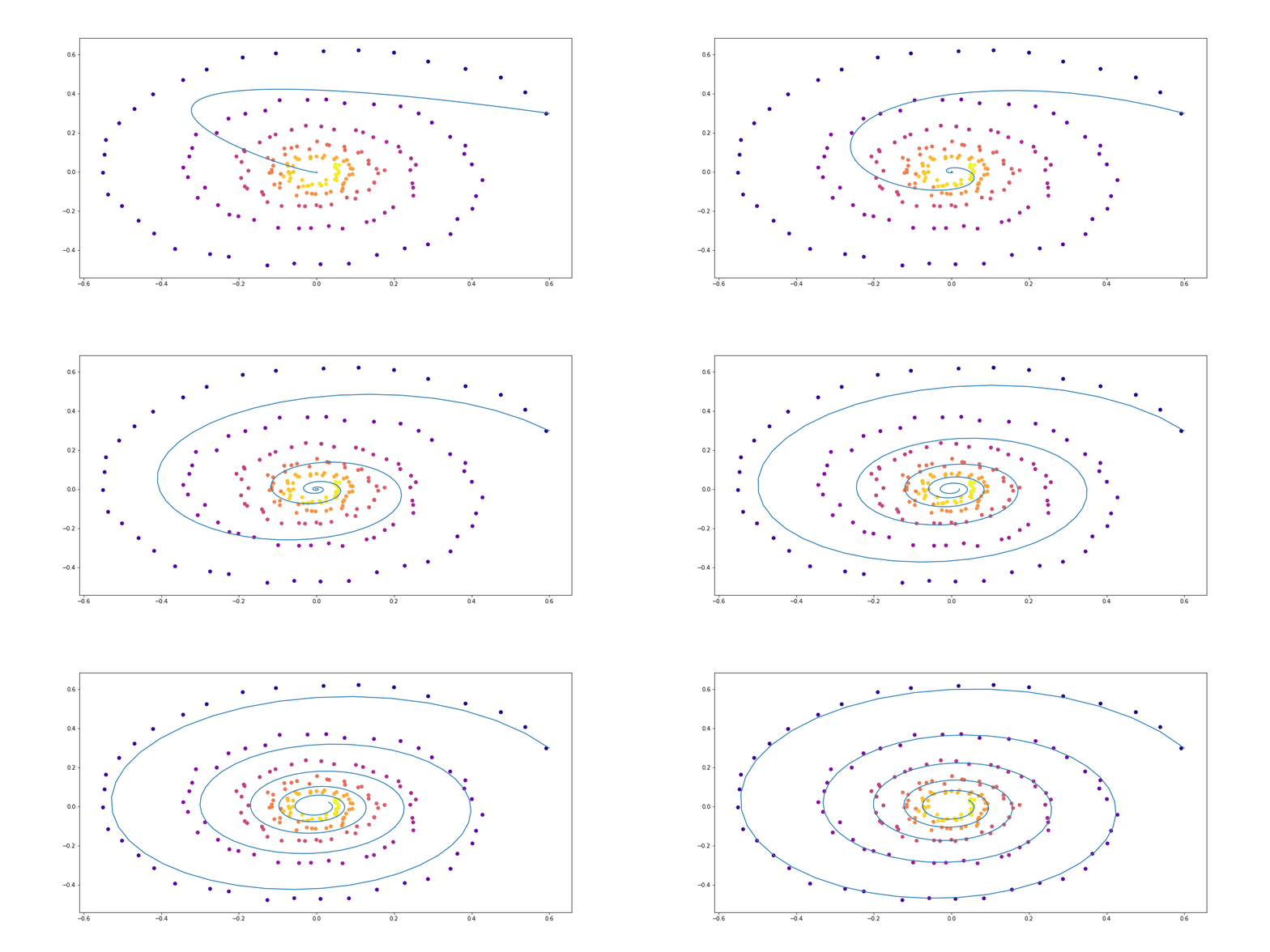
Further, a little more sophisticated dynamics (without a GIF, because the learning process is not so beautiful :))
The function taught here is a fully-connected network with one hidden layer.

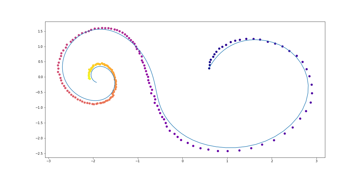
The code

class LinearODEF(ODEF):
    def __init__(self, W):
        super(LinearODEF, self).__init__()
        self.lin = nn.Linear(2, 2, bias=False)
        self.lin.weight = nn.Parameter(W)
    def forward(self, x, t):
        return self.lin(x)

The dynamics function is just a matrix

class SpiralFunctionExample(LinearODEF):
    def __init__(self):
        matrix = Tensor([[-0.1, -1.], [1., -0.1]])
        super(SpiralFunctionExample, self).__init__(matrix)

Randomly parameterized matrix

class RandomLinearODEF(LinearODEF):
    def __init__(self):
        super(RandomLinearODEF, self).__init__(torch.randn(2, 2)/2.)

Dynamics for more sophisticated trajectories

class TestODEF(ODEF):
    def __init__(self, A, B, x0):
        super(TestODEF, self).__init__()
        self.A = nn.Linear(2, 2, bias=False)
        self.A.weight = nn.Parameter(A)
        self.B = nn.Linear(2, 2, bias=False)
        self.B.weight = nn.Parameter(B)
        self.x0 = nn.Parameter(x0)
    def forward(self, x, t):
        xTx0 = torch.sum(x*self.x0, dim=1)
        dxdt = torch.sigmoid(xTx0) * self.A(x - self.x0) + 
               torch.sigmoid(-xTx0) * self.B(x + self.x0)
        return dxdt

Learning dynamics in the form of a fully connected network

class NNODEF(ODEF):
    def __init__(self, in_dim, hid_dim, time_invariant=False):
        super(NNODEF, self).__init__()
        self.time_invariant = time_invariant
        if time_invariant:
            self.lin1 = nn.Linear(in_dim, hid_dim)
        else:
            self.lin1 = nn.Linear(in_dim+1, hid_dim)
        self.lin2 = nn.Linear(hid_dim, hid_dim)
        self.lin3 = nn.Linear(hid_dim, in_dim)
        self.elu = nn.ELU(inplace=True)
    def forward(self, x, t):
        if not self.time_invariant:
            x = torch.cat((x, t), dim=-1)
        h = self.elu(self.lin1(x))
        h = self.elu(self.lin2(h))
        out = self.lin3(h)
        return out
def to_np(x):
    return x.detach().cpu().numpy()
def plot_trajectories(obs=None, times=None, trajs=None, save=None, figsize=(16, 8)):
    plt.figure(figsize=figsize)
    if obs is not None:
        if times is None:
            times = [None] * len(obs)
        for o, t in zip(obs, times):
            o, t = to_np(o), to_np(t)
            for b_i in range(o.shape[1]):
                plt.scatter(o[:, b_i, 0], o[:, b_i, 1], c=t[:, b_i, 0],
                            cmap=cm.plasma)
    if trajs is not None: 
        for z in trajs:
            z = to_np(z)
            plt.plot(z[:, 0, 0], z[:, 0, 1], lw=1.5)
        if save is not None:
            plt.savefig(save)
    plt.show()
def conduct_experiment(ode_true, ode_trained, n_steps, name, plot_freq=10):
    # Create data
    z0 = Variable(torch.Tensor([[0.6, 0.3]]))
    t_max = 6.29*5
    n_points = 200
    index_np = np.arange(0, n_points, 1, dtype=np.int)
    index_np = np.hstack([index_np[:, None]])
    times_np = np.linspace(0, t_max, num=n_points)
    times_np = np.hstack([times_np[:, None]])
    times = torch.from_numpy(times_np[:, :, None]).to(z0)
    obs = ode_true(z0, times, return_whole_sequence=True).detach()
    obs = obs + torch.randn_like(obs) * 0.01
    # Get trajectory of random timespan 
    min_delta_time = 1.0
    max_delta_time = 5.0
    max_points_num = 32
    def create_batch():
        t0 = np.random.uniform(0, t_max - max_delta_time)
        t1 = t0 + np.random.uniform(min_delta_time, max_delta_time)
        idx = sorted(np.random.permutation(
                  index_np[(times_np > t0) & (times_np < t1)]
              )[:max_points_num])
        obs_ = obs[idx]
        ts_ = times[idx]
        return obs_, ts_
    # Train Neural ODE
    optimizer = torch.optim.Adam(ode_trained.parameters(), lr=0.01)
    for i in range(n_steps):
        obs_, ts_ = create_batch()
        z_ = ode_trained(obs_[0], ts_, return_whole_sequence=True)
        loss = F.mse_loss(z_, obs_.detach())
        optimizer.zero_grad()
        loss.backward(retain_graph=True)
        optimizer.step()
        if i % plot_freq == 0:
            z_p = ode_trained(z0, times, return_whole_sequence=True)
            plot_trajectories(obs=[obs], times=[times], trajs=[z_p], 
                              save=f"assets/imgs/{name}/{i}.png")
            clear_output(wait=True)
ode_true = NeuralODE(SpiralFunctionExample())
ode_trained = NeuralODE(RandomLinearODEF())
conduct_experiment(ode_true, ode_trained, 500, "linear")
func = TestODEF(Tensor([[-0.1, -0.5], [0.5, -0.1]]),
                Tensor([[0.2, 1.], [-1, 0.2]]), Tensor([[-1., 0.]]))
ode_true = NeuralODE(func)
func = NNODEF(2, 16, time_invariant=True)
ode_trained = NeuralODE(func)
conduct_experiment(ode_true, ode_trained, 3000, "comp", plot_freq=30)

As you can see, Neural ODE does a pretty good job of restoring dynamics. That is, the concept as a whole works.
Now let's check on a slightly more complicated problem (MNIST, haha).

Neural ODE inspired by ResNets

In ResNet'ax, the latent state changes according to the formula

$h_ {t + 1} = h_ {t} + f (h_ {t}, \ theta_ {t})$

where $t \ in \ {0 ... T \}$ is the block number and

this is the function learned by the layers inside the block.

In the limit, if we take an infinite number of blocks with ever smaller steps, we get the continuous dynamics of the hidden layer in the form of an ODE, just like what was above.

$\ frac {dh (t)} {dt} = f (h (t), t, \ theta)$

Starting from the input layer h (0)

, we can define the output layer h (T)

as the solution of the TAC at time T.

We can now consider $\ theta$ as distributed ( shared ) between all parameters infinitely small blocks.

Validating Neural ODE Architecture on MNIST

In this part, we will test the ability of Neural ODE to be used as components in more familiar architectures.

In particular, we replace the remaining ( residual ) blocks on Neural ODE in the classifier MNIST.

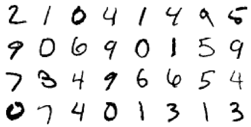
The code

def norm(dim):
    return nn.BatchNorm2d(dim)
def conv3x3(in_feats, out_feats, stride=1):
    return nn.Conv2d(in_feats, out_feats, kernel_size=3,
                     stride=stride, padding=1, bias=False)
def add_time(in_tensor, t):
    bs, c, w, h = in_tensor.shape
    return torch.cat((in_tensor, t.expand(bs, 1, w, h)), dim=1)
class ConvODEF(ODEF):
    def __init__(self, dim):
        super(ConvODEF, self).__init__()
        self.conv1 = conv3x3(dim + 1, dim)
        self.norm1 = norm(dim)
        self.conv2 = conv3x3(dim + 1, dim)
        self.norm2 = norm(dim)
    def forward(self, x, t):
        xt = add_time(x, t)
        h = self.norm1(torch.relu(self.conv1(xt)))
        ht = add_time(h, t)
        dxdt = self.norm2(torch.relu(self.conv2(ht)))
        return dxdt
class ContinuousNeuralMNISTClassifier(nn.Module):
    def __init__(self, ode):
        super(ContinuousNeuralMNISTClassifier, self).__init__()
        self.downsampling = nn.Sequential(
            nn.Conv2d(1, 64, 3, 1),
            norm(64),
            nn.ReLU(inplace=True),
            nn.Conv2d(64, 64, 4, 2, 1),
            norm(64),
            nn.ReLU(inplace=True),
            nn.Conv2d(64, 64, 4, 2, 1),
        )
        self.feature = ode
        self.norm = norm(64)
        self.avg_pool = nn.AdaptiveAvgPool2d((1, 1))
        self.fc = nn.Linear(64, 10)
    def forward(self, x):
        x = self.downsampling(x)
        x = self.feature(x)
        x = self.norm(x)
        x = self.avg_pool(x)
        shape = torch.prod(torch.tensor(x.shape[1:])).item()
        x = x.view(-1, shape)
        out = self.fc(x)
        return out
func = ConvODEF(64)
ode = NeuralODE(func)
model = ContinuousNeuralMNISTClassifier(ode)
if use_cuda:
    model = model.cuda()
import torchvision
img_std = 0.3081
img_mean = 0.1307
batch_size = 32
train_loader = torch.utils.data.DataLoader(
    torchvision.datasets.MNIST("data/mnist", train=True, download=True,
                             transform=torchvision.transforms.Compose([
                                 torchvision.transforms.ToTensor(),
                                 torchvision.transforms.Normalize((img_mean,),
                                                                  (img_std,))
                             ])
    ),
    batch_size=batch_size, shuffle=True
)
test_loader = torch.utils.data.DataLoader(
    torchvision.datasets.MNIST("data/mnist", train=False, download=True,
                             transform=torchvision.transforms.Compose([
                                 torchvision.transforms.ToTensor(),
                                 torchvision.transforms.Normalize((img_mean,),
                                                                  (img_std,))
                             ])
    ),
    batch_size=128, shuffle=True
)
optimizer = torch.optim.Adam(model.parameters())
def train(epoch):
    num_items = 0
    train_losses = []
    model.train()
    criterion = nn.CrossEntropyLoss()
    print(f"Training Epoch {epoch}...")
    for batch_idx, (data, target) in tqdm(enumerate(train_loader),
                                          total=len(train_loader)):
        if use_cuda:
            data = data.cuda()
            target = target.cuda()
        optimizer.zero_grad()
        output = model(data)
        loss = criterion(output, target) 
        loss.backward()
        optimizer.step()
        train_losses += [loss.item()]
        num_items += data.shape[0]
    print('Train loss: {:.5f}'.format(np.mean(train_losses)))
    return train_losses
def test():
    accuracy = 0.0
    num_items = 0
    model.eval()
    criterion = nn.CrossEntropyLoss()
    print(f"Testing...")
    with torch.no_grad():
        for batch_idx, (data, target) in tqdm(enumerate(test_loader),
                                              total=len(test_loader)):
            if use_cuda:
                data = data.cuda()
                target = target.cuda()
            output = model(data)
            accuracy += torch.sum(torch.argmax(output, dim=1) == target).item()
            num_items += data.shape[0]
    accuracy = accuracy * 100 / num_items
    print("Test Accuracy: {:.3f}%".format(accuracy))
n_epochs = 5
test()
train_losses = []
for epoch in range(1, n_epochs + 1):
    train_losses += train(epoch)
    test()
import pandas as pd
plt.figure(figsize=(9, 5))
history = pd.DataFrame({"loss": train_losses})
history["cum_data"] = history.index * batch_size
history["smooth_loss"] = history.loss.ewm(halflife=10).mean()
history.plot(x="cum_data", y="smooth_loss", figsize=(12, 5), title="train error")

Testing...
100% 79/79 [00:01<00:00, 45.69it/s]
Test Accuracy: 9.740%
Training Epoch 1...
100% 1875/1875 [01:15<00:00, 24.69it/s]
Train loss: 0.20137
Testing...
100% 79/79 [00:01<00:00, 46.64it/s]
Test Accuracy: 98.680%
Training Epoch 2...
100% 1875/1875 [01:17<00:00, 24.32it/s]
Train loss: 0.05059
Testing...
100% 79/79 [00:01<00:00, 46.11it/s]
Test Accuracy: 97.760%
Training Epoch 3...
100% 1875/1875 [01:16<00:00, 24.63it/s]
Train loss: 0.03808
Testing...
100% 79/79 [00:01<00:00, 45.65it/s]
Test Accuracy: 99.000%
Training Epoch 4...
100% 1875/1875 [01:17<00:00, 24.28it/s]
Train loss: 0.02894
Testing...
100% 79/79 [00:01<00:00, 45.42it/s]
Test Accuracy: 99.130%
Training Epoch 5...
100% 1875/1875 [01:16<00:00, 24.67it/s]
Train loss: 0.02424
Testing...
100% 79/79 [00:01<00:00, 45.89it/s]
Test Accuracy: 99.170%

After a very rough training during just 5 eras and 6 minutes of training, the model has already reached a test error of less than 1%. It can be said that Neural ODEs integrate well as a component into more traditional networks.

In their article, the authors also compare this classifier (ODE-Net) with a regular fully-connected network, with ResNet with a similar architecture, and with the exact same architecture, in which the gradient propagates directly through operations in ODESolve (without the conjugate gradient method) ( RK-Net).

Illustration from the original article

According to them, a 1-layer fully connected network with approximately the same number of parameters as Neural ODE has a much higher error in the test, ResNet with approximately the same error has much more parameters, and RK-Net without the conjugate gradient method has a slightly higher error and with a linearly increasing memory consumption (the smaller the permissible error, the more steps ODESolve must take , which linearly increases the memory consumption with the number of steps).

The authors use the implicit Runge-Kutta method with adaptive step size in their implementation, unlike the simpler Euler method here. They also study some features of the new architecture.

Характеристика ODE-Net (NFE Forward — количество вычислений функции при прямом проходе)
Иллюстрация из оригинальной статьи

(a) Изменение допустимого уровня численной ошибки изменяет количество шагов в прямом распространении.
(b) Время потраченное на прямое распространение пропорционально количеству вычислений функции.
(с) Количество вычислений функции при обратном распространение составляет примерно половину от прямого распространения, это указывает на то, что метод сопряженного градиента может быть более вычислительно эффективным, чем распространение градиента напрямую через ODESolve.
(d) Как ODE-Net становится все более и более обученным, он требует все больше вычислений функции (все меньший шаг), возможно адаптируясь под возрастающую сложность модели.

Hidden Generative Function for Time Series Modeling

Neural ODE is suitable for processing continuous serial data even when the trajectory lies in an unknown hidden space.

In this section, we will experiment and change the generation of continuous sequences using Neural ODE , and take a look at the learned hidden space.

The authors also compare it with a similar sequence s , generated by recurrent networks.

The experiment here is slightly different from the corresponding example in the authors repository, here there is a more diverse set of trajectories.

Data

The training data consists of random spirals, half of which are clockwise, and the second counterclockwise. Further, random subsequences are sampled from these spirals, processed by the coding recursive model in the opposite direction, generating a starting latent state, which then evolves, creating a trajectory in the hidden space. This latent path is then mapped to the data space and compared with the sampled subsequence. Thus, the model learns to generate trajectories similar to a dataset.

Examples of dataset spirals

VAE as a generative model

Generative model through a sampling procedure:

$z_ {t_0} \ sim \ mathcal {N} (0, I)$

$z_ {t_1}, z_ {t_2}, ..., z_ {t_M} = \ text {ODESolve} (z_ {t_0}, f, \ theta_f, t_0, ..., t_M)$

$x_ {t_i} \ sim p (x \ mid z_ {t_i}; \ theta_x)$

Which can be trained using the variational auto-encoder approach.

Go through the recurrent encoder through the time sequence back in time to get the parameters $\ mu_ {z_ {t_0}}$ , the $\ sigma_ {z_ {t_0}}$ variational posterior distribution, and then sample from it:

$z_{t_0} \sim q \left( z_{t_0} \mid x_{t_0},...,x_{t_M}; t_0,...,t_M; \theta_q \right) = \mathcal{N} \left(z_{t_0} \mid \mu_{z_{t_0}} \sigma_{z_{t_0}} \right)$

Get hidden trajectory:

$z_{t_1}, z_{t_2},...,z_{t_N} = \text{ODESolve}(z_{t_0}, f, \theta_f, t_0,...,t_N), \text{ где } \frac{d z}{d t} = f(z, t; \theta_f)$

Map a hidden path to a path in the data using another neural network: $\hat{x_{t_i}}(z_{t_i}, t_i; \theta_x)$
Maximize the assessment of the lower bound of validity (ELBO) for the sampled path:

$\text{ELBO} \approx N \Big( \sum_{i=0}^{M} \log p(x_{t_i} \mid z_{t_i}(z_{t_0}; \theta_f); \theta_x) + KL \left( q( z_{t_0} \mid x_{t_0},...,x_{t_M}; t_0,...,t_M; \theta_q) \parallel \mathcal{N}(0, I) \right) \Big)$

And in the case of a Gaussian posterior distribution $p(x \mid z_{t_i};\theta_x)$ and a known noise level $\sigma_x$ :

$\text{ELBO} \approx -N \Big( \sum_{i=1}^{M}\frac{(x_i - \hat{x_i} )^2}{\sigma_x^2} - \log \sigma_{z_{t_0}}^2 + \mu_{z_{t_0}}^2 + \sigma_{z_{t_0}}^2 \Big) + C$

The computation graph of a hidden ODE model can be represented as follows

Illustration from the original article

This model can then be tested for how it interpolates the path using only the initial observations.

The code

Define models

class RNNEncoder(nn.Module):
    def __init__(self, input_dim, hidden_dim, latent_dim):
        super(RNNEncoder, self).__init__()
        self.input_dim = input_dim
        self.hidden_dim = hidden_dim
        self.latent_dim = latent_dim
        self.rnn = nn.GRU(input_dim+1, hidden_dim)
        self.hid2lat = nn.Linear(hidden_dim, 2*latent_dim)
    def forward(self, x, t):
        # Concatenate time to input
        t = t.clone()
        t[1:] = t[:-1] - t[1:]
        t[0] = 0.
        xt = torch.cat((x, t), dim=-1)
        _, h0 = self.rnn(xt.flip((0,)))  # Reversed
        # Compute latent dimension
        z0 = self.hid2lat(h0[0])
        z0_mean = z0[:, :self.latent_dim]
        z0_log_var = z0[:, self.latent_dim:]
        return z0_mean, z0_log_var
class NeuralODEDecoder(nn.Module):
    def __init__(self, output_dim, hidden_dim, latent_dim):
        super(NeuralODEDecoder, self).__init__()
        self.output_dim = output_dim
        self.hidden_dim = hidden_dim
        self.latent_dim = latent_dim
        func = NNODEF(latent_dim, hidden_dim, time_invariant=True)
        self.ode = NeuralODE(func)
        self.l2h = nn.Linear(latent_dim, hidden_dim)
        self.h2o = nn.Linear(hidden_dim, output_dim)
    def forward(self, z0, t):
        zs = self.ode(z0, t, return_whole_sequence=True)
        hs = self.l2h(zs)
        xs = self.h2o(hs)
        return xs
class ODEVAE(nn.Module):
    def __init__(self, output_dim, hidden_dim, latent_dim):
        super(ODEVAE, self).__init__()
        self.output_dim = output_dim
        self.hidden_dim = hidden_dim
        self.latent_dim = latent_dim
        self.encoder = RNNEncoder(output_dim, hidden_dim, latent_dim)
        self.decoder = NeuralODEDecoder(output_dim, hidden_dim, latent_dim)
    def forward(self, x, t, MAP=False):
        z_mean, z_log_var = self.encoder(x, t)
        if MAP:
            z = z_mean
        else:
            z = z_mean + torch.randn_like(z_mean) * torch.exp(0.5 * z_log_var)
        x_p = self.decoder(z, t)
        return x_p, z, z_mean, z_log_var
    def generate_with_seed(self, seed_x, t):
        seed_t_len = seed_x.shape[0]
        z_mean, z_log_var = self.encoder(seed_x, t[:seed_t_len])
        x_p = self.decoder(z_mean, t)
        return x_p

Dataset generation

t_max = 6.29*5
n_points = 200
noise_std = 0.02
num_spirals = 1000
index_np = np.arange(0, n_points, 1, dtype=np.int)
index_np = np.hstack([index_np[:, None]])
times_np = np.linspace(0, t_max, num=n_points)
times_np = np.hstack([times_np[:, None]] * num_spirals)
times = torch.from_numpy(times_np[:, :, None]).to(torch.float32)
# Generate random spirals parameters
normal01 = torch.distributions.Normal(0, 1.0)
x0 = Variable(normal01.sample((num_spirals, 2))) * 2.0  
W11 = -0.1 * normal01.sample((num_spirals,)).abs() - 0.05
W22 = -0.1 * normal01.sample((num_spirals,)).abs() - 0.05
W21 = -1.0 * normal01.sample((num_spirals,)).abs()
W12 =  1.0 * normal01.sample((num_spirals,)).abs()
xs_list = []
for i in range(num_spirals):
    if i % 2 == 1: #  Make it counter-clockwise
        W21, W12 = W12, W21
    func = LinearODEF(Tensor([[W11[i], W12[i]], [W21[i], W22[i]]]))
    ode = NeuralODE(func)
    xs = ode(x0[i:i+1], times[:, i:i+1], return_whole_sequence=True)
    xs_list.append(xs)
orig_trajs = torch.cat(xs_list, dim=1).detach()
samp_trajs = orig_trajs + torch.randn_like(orig_trajs) * noise_std
samp_ts = times
fig, axes = plt.subplots(nrows=3, ncols=3, figsize=(15, 9))
axes = axes.flatten()
for i, ax in enumerate(axes):
    ax.scatter(samp_trajs[:, i, 0], samp_trajs[:, i, 1], c=samp_ts[:, i, 0],
               cmap=cm.plasma)
plt.show()
import numpy.random as npr
def gen_batch(batch_size, n_sample=100):
    n_batches = samp_trajs.shape[1] // batch_size
    time_len = samp_trajs.shape[0]
    n_sample = min(n_sample, time_len)
    for i in range(n_batches):
        if n_sample > 0:
            probs = [1. / (time_len - n_sample)] * (time_len - n_sample)
            t0_idx = npr.multinomial(1, probs)
            t0_idx = np.argmax(t0_idx)
            tM_idx = t0_idx + n_sample
        else:
            t0_idx = 0
            tM_idx = time_len
        frm, to = batch_size*i, batch_size*(i+1)
        yield samp_trajs[t0_idx:tM_idx, frm:to], samp_ts[t0_idx:tM_idx, frm:to]

Training

vae = ODEVAE(2, 64, 6)
vae = vae.cuda()
if use_cuda:
    vae = vae.cuda()
optim = torch.optim.Adam(vae.parameters(), betas=(0.9, 0.999), lr=0.001)
preload = False
n_epochs = 20000
batch_size = 100
plot_traj_idx = 1
plot_traj = orig_trajs[:, plot_traj_idx:plot_traj_idx+1]
plot_obs = samp_trajs[:, plot_traj_idx:plot_traj_idx+1]
plot_ts = samp_ts[:, plot_traj_idx:plot_traj_idx+1]
if use_cuda:
    plot_traj = plot_traj.cuda()
    plot_obs = plot_obs.cuda()
    plot_ts = plot_ts.cuda()
if preload:
    vae.load_state_dict(torch.load("models/vae_spirals.sd"))
for epoch_idx in range(n_epochs):
    losses = []
    train_iter = gen_batch(batch_size)
    for x, t in train_iter:
        optim.zero_grad()
        if use_cuda:
            x, t = x.cuda(), t.cuda()
        max_len = np.random.choice([30, 50, 100])
        permutation = np.random.permutation(t.shape[0])
        np.random.shuffle(permutation)
        permutation = np.sort(permutation[:max_len])
        x, t = x[permutation], t[permutation]
        x_p, z, z_mean, z_log_var = vae(x, t)
        z_var = torch.exp(z_log_var)
        kl_loss = -0.5 * torch.sum(1 + z_log_var - z_mean**2 - z_var, -1)
        loss = 0.5 * ((x-x_p)**2).sum(-1).sum(0) / noise_std**2 + kl_loss
        loss = torch.mean(loss)
        loss /= max_len
        loss.backward()
        optim.step()
        losses.append(loss.item())
    print(f"Epoch {epoch_idx}")
    frm, to, to_seed = 0, 200, 50
    seed_trajs = samp_trajs[frm:to_seed]
    ts = samp_ts[frm:to]
    if use_cuda:
        seed_trajs = seed_trajs.cuda()
        ts = ts.cuda()
    samp_trajs_p = to_np(vae.generate_with_seed(seed_trajs, ts))
    fig, axes = plt.subplots(nrows=3, ncols=3, figsize=(15, 9))
    axes = axes.flatten()
    for i, ax in enumerate(axes):
        ax.scatter(to_np(seed_trajs[:, i, 0]),
                   to_np(seed_trajs[:, i, 1]),
                   c=to_np(ts[frm:to_seed, i, 0]),
                   cmap=cm.plasma)
        ax.plot(to_np(orig_trajs[frm:to, i, 0]), to_np(orig_trajs[frm:to, i, 1]))
        ax.plot(samp_trajs_p[:, i, 0], samp_trajs_p[:, i, 1])
    plt.show()
    print(np.mean(losses), np.median(losses))
    clear_output(wait=True)
spiral_0_idx = 3
spiral_1_idx = 6
homotopy_p = Tensor(np.linspace(0., 1., 10)[:, None])
vae = vae
if use_cuda:
    homotopy_p = homotopy_p.cuda()
    vae = vae.cuda()
spiral_0 = orig_trajs[:, spiral_0_idx:spiral_0_idx+1, :]
spiral_1 = orig_trajs[:, spiral_1_idx:spiral_1_idx+1, :]
ts_0 = samp_ts[:, spiral_0_idx:spiral_0_idx+1, :]
ts_1 = samp_ts[:, spiral_1_idx:spiral_1_idx+1, :]
if use_cuda:
    spiral_0, ts_0 = spiral_0.cuda(), ts_0.cuda()
    spiral_1, ts_1 = spiral_1.cuda(), ts_1.cuda()
z_cw, _ = vae.encoder(spiral_0, ts_0)
z_cc, _ = vae.encoder(spiral_1, ts_1)
homotopy_z = z_cw * (1 - homotopy_p) + z_cc * homotopy_p
t = torch.from_numpy(np.linspace(0, 6*np.pi, 200))
t = t[:, None].expand(200, 10)[:, :, None].cuda()
t = t.cuda() if use_cuda else t
hom_gen_trajs = vae.decoder(homotopy_z, t)
fig, axes = plt.subplots(nrows=2, ncols=5, figsize=(15, 5))
axes = axes.flatten()
for i, ax in enumerate(axes):
    ax.plot(to_np(hom_gen_trajs[:, i, 0]), to_np(hom_gen_trajs[:, i, 1]))
plt.show()
torch.save(vae.state_dict(), "models/vae_spirals.sd")

That's what happens after a night of training

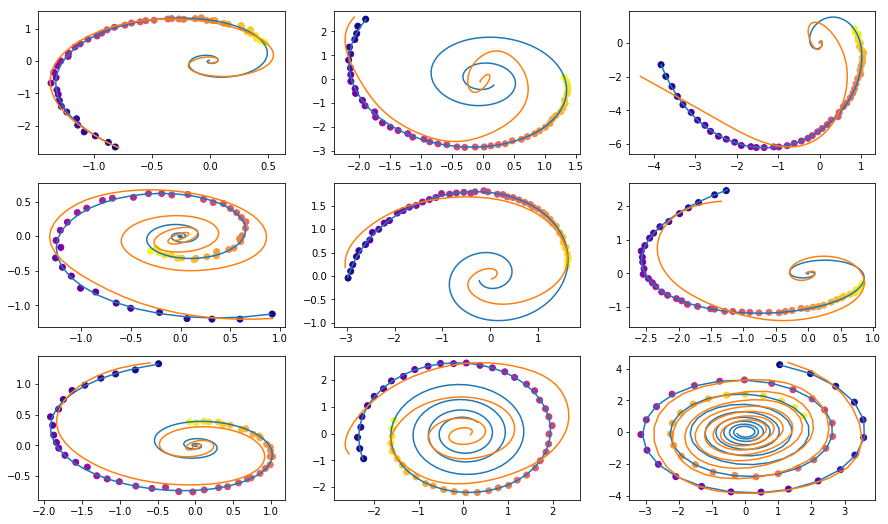
Points are noisy observations of the original trajectory (blue),
yellow are reconstructed and interpolated trajectories, using points as inputs.

The color of the dot shows time.

Reconstructions of some examples do not look too good. Maybe the model is not complex enough or not studied long enough. In any case, the reconstruction looks very reasonable.

Now let's see what happens if we interpolate a hidden variable in a clockwise trajectory to an anti-clockwise trajectory.

The authors also compare reconstructions and path interpolations between Neural ODE and a simple Recursive Network.

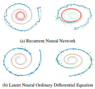
Illustration from the original article.

Continuous Normalizing Streams

The original article also brings a lot to the topic of Normalizing Streams. Normalizing flows are used when you need to sample from some complex distribution that appears through a change of variables from some simple distribution (Gaussian, for example), and still know the probability density at the point of each sample.
The authors show that using continuous variable substitution is much more computationally efficient and interpretable than previous methods.

Normalizing flows are very useful in models such as Variation AutoCoders , Bayesian Neural Networks and others from the Bayesian approach.

This topic, however, lies outside the scope of thisarticles, and those who are interested should read the original scientific article.

For seed:

Visualization of transformation from noise (simple distribution) to data (complex distribution) for two datasets;

The X-axis shows the transformation of density and samples over the course of “time” (for NS) and “depth” (for NS).

Illustration from the original article

Thanks to bekemax for help in editing the English version of the text and for interesting physical comments.

This concludes my little research on Neural ODEs . Thanks for attention!

useful links

Tags:

Introducing Neural ODE

Neural Ordinary Differential Equations

Formulation of the problem

Implementation

Application

Recovery of the real dynamics function (approach verification)

Neural ODE inspired by ResNets

Validating Neural ODE Architecture on MNIST

Hidden Generative Function for Time Series Modeling

Data

VAE as a generative model

Define models

Dataset generation

Training

Continuous Normalizing Streams

useful links

Also popular now: