Machine-synesthetic approach to detecting network DDoS attacks. Part 2
- Transfer
Hello again. Today we continue to share material dedicated to the launch of the course "Network Engineer" , which starts already in early March. We see that many were interested in the first part of the article “Machine-synesthetic approach to detecting network DDoS attacks” and today we want to share with you the second - the final part.
3.2 Classification of images in the problem of detection of anomalies
The next step is to solve the problem of classification of the received image. In general, the solution to the problem of detecting classes (objects) in an image is to use machine learning algorithms to build class models, and then algorithms to search for classes (objects) in an image.

Building a model consists of two stages:
a) Feature extraction for a class: plot feature vectors for class members.
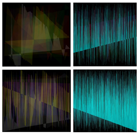
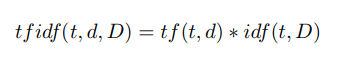
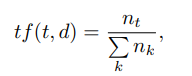
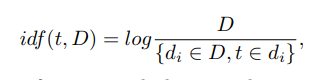
Fig. 1
b) Training in the obtained model features for subsequent recognition tasks.
The class object is described using feature vectors. Vectors are formed from:
a) color information (oriented gradient histogram);
b) contextual information;
c) data on the geometric arrangement of parts of the object.
The classification (forecasting) algorithm can be divided into two stages:
a) Extract features from the image. At this stage, two tasks are performed:
b) associating an image with a particular class. A formal description of the class, that is, a set of features that are highlighted by their test images, is used as input. Based on this information, the classifier decides whether the image belongs to the class and evaluates the degree of certainty for the conclusion.
Classification Methods. Classification methods range from predominantly heuristic approaches to formal procedures based on methods of mathematical statistics. There is no generally accepted classification, but several approaches to image classification can be distinguished:
For the implementation presented in this article, the authors chose the “word bag” algorithm, given the following reasons:
To analyze the video stream projected from the traffic, we used the naive Bayes classifier [25]. It is often used to classify texts using the word bag model. In this case, the approach is similar to text analysis, instead of words only descriptors are used. The work of this classifier can be divided into two parts: the training phase and the forecasting phase.
Learning phase . Each frame (image) is fed to the input of the descriptor search algorithm, in this case, the scale-invariant feature transform (SIFT) [26]. After that, the task of correlation of singular points between frames is performed. A particular point in the image of an object is a point that is likely to appear on other images of this object.
To solve the problem of comparing special points of an object in different images, a descriptor is used. A descriptor is a data structure, an identifier for a singular point that distinguishes it from the rest. It may or may not be invariant with respect to transformations of the image of the object. In our case, the descriptor is invariant with respect to perspective transformations, i.e. scaling. The handle allows you to compare the feature point of an object in one image with the same feature point in another image of this object.
Then, the set of descriptors obtained from all images is sorted into groups by similarity using the k-means clustering method [26, 27]. This is done in order to train the classifier, which will give a conclusion on whether the image represents an abnormal behavior.
The following is a step-by-step algorithm for training the image descriptor classifier:
Step 1 . Extract all descriptors from sets with and without attack.
Step 2 . Clustering all descriptors using the k-means method in n clusters.
Step 3 . Calculation of the matrix A (m, k), where m is the number of images and k is the number of clusters. The element (i; j) will store the value of how often descriptors from the j-th cluster appear on the i-th image. Such a matrix will be called the matrix of the frequency of occurrence.
Step 4 . Calculation of descriptor weights using the formula tf idf [28]:
Here tf (“term frequency”) is the frequency of appearance of the descriptor in this image and is defined as
where t is the descriptor, k is the number of descriptors in the image, nt is the number of descriptors t in the image. In addition, idf (“inverse document frequency”) is the inverse frequency of the image with the given descriptor in the sample and is defined as
where D is the number of images with the given descriptor in the sample, {di ∈ D, t ∈ di} is the number of images in D, where t is in nt! = 0.
Step 5 . Substituting the corresponding weights instead of descriptors in matrix A.
Step 6 . Classification. We use amplification of naive Bayes classifiers (adaboost).
Step 7 . Saving the trained model to a file.
Step 8 . This concludes the training phase.
Prediction phase. The differences between the training phase and the forecasting phase are small: descriptors are extracted from the image and correlated with the existing groups. Based on this ratio, a vector is constructed. Each element of this vector is the frequency of appearance of descriptors from this group in the image. By analyzing this vector, the classifier can make an attack forecast with a certain probability.
A general forecasting algorithm based on a pair of classifiers is presented below.
Step 1 . Extract all descriptors from the image;
Step 2 . Clustering the resulting set of descriptors;
Step 3 . Calculation of the vector [1, k];
Step 4 . Calculation of the weight for each descriptor according to the formula tf idf presented above;
Step 5. Replacing the frequency of occurrence in vectors with their weight;
Step 6 . Classification of the resulting vector according to a previously trained classifier;
Step 7 . Conclusion about the presence of anomalies in the observed network based on the forecast of the classifier.
4. Evaluation of the effectiveness of detection
The task of evaluating the effectiveness of the proposed method was solved experimentally. In the experiment, a number of parameters established experimentally were used. For clustering, 1000 clusters were used. The generated images had 1000 by 1000 pixels.
4.1 Experimental data set
For experiments, a setup was assembled. It consists of three devices connected by a communication channel. The installation block diagram is shown in Figure 2.
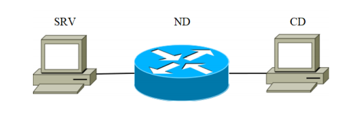
Fig . 1
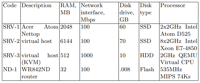
The SRV device acts as the attacking server (hereinafter referred to as the target server). The devices listed in Table 1 with the SRV code were sequentially used as the target server. The second is a network device designed to transmit network packets. The characteristics of the device are shown in Table 1 under the code ND-1.
Table 1. Network device characteristics
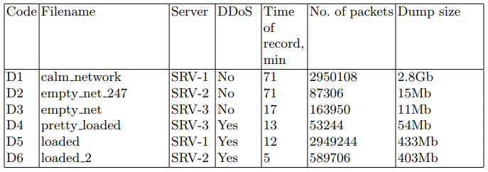
On the target servers, network packets were written to a PCAP file for later use in discovery algorithms. The tcpdump utility was used for this task. The data sets are described in Table 2.
Table 2. Sets of intercepted network packets
The following software was used on the target servers: Linux distribution, nginx 1.10.3 web server, postgresql 9.6 DBMS. A special web application was written to emulate system boot. The application requests a database with a large amount of data. The request is designed to minimize the use of various caching. During the experiments, requests for this web application were generated.
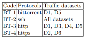
The attack was made from the third client device (table 1) using the Apache Benchmark utility. The structure of background traffic during the attack and the rest of the time is presented in Table 3.
Table 3. Background traffic functions
As an attack, we implement the distributed DoS version of the HTTP GET flood. Such an attack, in fact, is the generation of a constant stream of GET requests, in this case from a CD-1 device. To generate it, we used the ab utility from the apache-utils package. As a result, files containing information about the status of the network were received. The main characteristics of these files are presented in Table 2. The main parameters of the attack scenario are shown in Table 4.
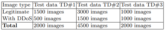
From the obtained network traffic dump, sets of generated images TD # 1 and TD # 2 were obtained, which were used at the training stage. Sample TD # 3 was used for the prediction phase. A summary of the test data sets is presented in Table 5.
4.2 Performance criteria
The main parameters evaluated during this study were:
Table 4. Features of DDoS attacks
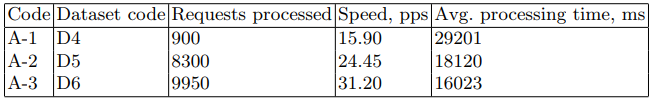
Table 5. Test image sets a
) DR (Detection Rate) - the number of detected attacks in relation to the total number of attacks. The higher this parameter, the higher the efficiency and quality of ADS.
b) FPR (False Positive Rate) - the number of “normal” objects, erroneously classified as an attack, in relation to the total number of “normal” objects. The lower this parameter, the higher the efficiency and quality of the anomaly detection system.
c) CR (Complex rate) is a complex indicator that takes into account the combination of DR and FPR parameters. Since the parameters DR and FPR were taken equal in importance in the study, the complex indicator was calculated as follows: CR = (DR + FPR) / 2.
1000 images marked as "abnormal" were submitted to the classifier. Based on the recognition results, DR was calculated depending on the size of the training sample. The following values were obtained: for TD # 1 DR = 9.5% and for TD # 2 DR = 98.4%. Further, the second half of the images (“normal”) were classified. Based on the result, FPR was calculated (for TD # 1 FPR = 3.2% and for TD # 2 FPR = 4.3%). Thus, the following comprehensive performance indicators were obtained: for TD # 1 CR = 53.15% and for TD # 2 CR = 97.05%.
5. Conclusions and future research
From the experimental results it is seen that the proposed method for detecting anomalies shows high results in detecting attacks. For example, in a large sample, the value of a comprehensive performance indicator reaches 97%. However, this method has some limitations in application:
1. The DR and FPR values show the sensitivity of the algorithm to the size of the training set, which is a conceptual problem for machine learning algorithms. Increasing the sample improves detection performance. However, it is not always possible to implement a sufficiently large training set for a particular network.
2. The developed algorithm is deterministic, the same image is classified each time with the same result.
3. The effectiveness indicators of the approach are good enough to confirm the concept, but the number of false positives is also large, which can lead to difficulties in practical implementation.
In order to overcome the limitation described above (point 3), it is supposed to change the naive Bayesian classifier to a convolutional neural network, which, according to the authors, should increase the accuracy of the anomaly detection algorithm.
Traditionally, we are waiting for your comments and we invite everyone to an open day , which will be held next Monday.
3.2 Classification of images in the problem of detection of anomalies
The next step is to solve the problem of classification of the received image. In general, the solution to the problem of detecting classes (objects) in an image is to use machine learning algorithms to build class models, and then algorithms to search for classes (objects) in an image.
Building a model consists of two stages:
a) Feature extraction for a class: plot feature vectors for class members.
Fig. 1
b) Training in the obtained model features for subsequent recognition tasks.
The class object is described using feature vectors. Vectors are formed from:
a) color information (oriented gradient histogram);
b) contextual information;
c) data on the geometric arrangement of parts of the object.
The classification (forecasting) algorithm can be divided into two stages:
a) Extract features from the image. At this stage, two tasks are performed:
- Since the image may contain objects of many classes, we need to find all the representatives. To do this, you can use a sliding window that passes through the image from the upper left to the lower right.
- The image is scaled because the scale of objects in the image can change.
b) associating an image with a particular class. A formal description of the class, that is, a set of features that are highlighted by their test images, is used as input. Based on this information, the classifier decides whether the image belongs to the class and evaluates the degree of certainty for the conclusion.
Classification Methods. Classification methods range from predominantly heuristic approaches to formal procedures based on methods of mathematical statistics. There is no generally accepted classification, but several approaches to image classification can be distinguished:
- methods of object modeling based on details;
- methods of the "bag of words";
- methods of matching spatial pyramids.
For the implementation presented in this article, the authors chose the “word bag” algorithm, given the following reasons:
- Algorithms for modeling based on details and matching spatial pyramids are sensitive to the position of the descriptors in space and their relative position. These classes of methods are effective in the tasks of detecting objects in an image; however, due to the characteristic features of the input data, they are poorly applicable to the problem of image classification.
- The “bag of words” algorithm has been widely tested in other fields of knowledge, it shows good results and is quite simple to implement.
To analyze the video stream projected from the traffic, we used the naive Bayes classifier [25]. It is often used to classify texts using the word bag model. In this case, the approach is similar to text analysis, instead of words only descriptors are used. The work of this classifier can be divided into two parts: the training phase and the forecasting phase.
Learning phase . Each frame (image) is fed to the input of the descriptor search algorithm, in this case, the scale-invariant feature transform (SIFT) [26]. After that, the task of correlation of singular points between frames is performed. A particular point in the image of an object is a point that is likely to appear on other images of this object.
To solve the problem of comparing special points of an object in different images, a descriptor is used. A descriptor is a data structure, an identifier for a singular point that distinguishes it from the rest. It may or may not be invariant with respect to transformations of the image of the object. In our case, the descriptor is invariant with respect to perspective transformations, i.e. scaling. The handle allows you to compare the feature point of an object in one image with the same feature point in another image of this object.
Then, the set of descriptors obtained from all images is sorted into groups by similarity using the k-means clustering method [26, 27]. This is done in order to train the classifier, which will give a conclusion on whether the image represents an abnormal behavior.
The following is a step-by-step algorithm for training the image descriptor classifier:
Step 1 . Extract all descriptors from sets with and without attack.
Step 2 . Clustering all descriptors using the k-means method in n clusters.
Step 3 . Calculation of the matrix A (m, k), where m is the number of images and k is the number of clusters. The element (i; j) will store the value of how often descriptors from the j-th cluster appear on the i-th image. Such a matrix will be called the matrix of the frequency of occurrence.
Step 4 . Calculation of descriptor weights using the formula tf idf [28]:
Here tf (“term frequency”) is the frequency of appearance of the descriptor in this image and is defined as
where t is the descriptor, k is the number of descriptors in the image, nt is the number of descriptors t in the image. In addition, idf (“inverse document frequency”) is the inverse frequency of the image with the given descriptor in the sample and is defined as
where D is the number of images with the given descriptor in the sample, {di ∈ D, t ∈ di} is the number of images in D, where t is in nt! = 0.
Step 5 . Substituting the corresponding weights instead of descriptors in matrix A.
Step 6 . Classification. We use amplification of naive Bayes classifiers (adaboost).
Step 7 . Saving the trained model to a file.
Step 8 . This concludes the training phase.
Prediction phase. The differences between the training phase and the forecasting phase are small: descriptors are extracted from the image and correlated with the existing groups. Based on this ratio, a vector is constructed. Each element of this vector is the frequency of appearance of descriptors from this group in the image. By analyzing this vector, the classifier can make an attack forecast with a certain probability.
A general forecasting algorithm based on a pair of classifiers is presented below.
Step 1 . Extract all descriptors from the image;
Step 2 . Clustering the resulting set of descriptors;
Step 3 . Calculation of the vector [1, k];
Step 4 . Calculation of the weight for each descriptor according to the formula tf idf presented above;
Step 5. Replacing the frequency of occurrence in vectors with their weight;
Step 6 . Classification of the resulting vector according to a previously trained classifier;
Step 7 . Conclusion about the presence of anomalies in the observed network based on the forecast of the classifier.
4. Evaluation of the effectiveness of detection
The task of evaluating the effectiveness of the proposed method was solved experimentally. In the experiment, a number of parameters established experimentally were used. For clustering, 1000 clusters were used. The generated images had 1000 by 1000 pixels.
4.1 Experimental data set
For experiments, a setup was assembled. It consists of three devices connected by a communication channel. The installation block diagram is shown in Figure 2.
Fig . 1
The SRV device acts as the attacking server (hereinafter referred to as the target server). The devices listed in Table 1 with the SRV code were sequentially used as the target server. The second is a network device designed to transmit network packets. The characteristics of the device are shown in Table 1 under the code ND-1.
Table 1. Network device characteristics
On the target servers, network packets were written to a PCAP file for later use in discovery algorithms. The tcpdump utility was used for this task. The data sets are described in Table 2.
Table 2. Sets of intercepted network packets
The following software was used on the target servers: Linux distribution, nginx 1.10.3 web server, postgresql 9.6 DBMS. A special web application was written to emulate system boot. The application requests a database with a large amount of data. The request is designed to minimize the use of various caching. During the experiments, requests for this web application were generated.
The attack was made from the third client device (table 1) using the Apache Benchmark utility. The structure of background traffic during the attack and the rest of the time is presented in Table 3.
Table 3. Background traffic functions
As an attack, we implement the distributed DoS version of the HTTP GET flood. Such an attack, in fact, is the generation of a constant stream of GET requests, in this case from a CD-1 device. To generate it, we used the ab utility from the apache-utils package. As a result, files containing information about the status of the network were received. The main characteristics of these files are presented in Table 2. The main parameters of the attack scenario are shown in Table 4.
From the obtained network traffic dump, sets of generated images TD # 1 and TD # 2 were obtained, which were used at the training stage. Sample TD # 3 was used for the prediction phase. A summary of the test data sets is presented in Table 5.
4.2 Performance criteria
The main parameters evaluated during this study were:
Table 4. Features of DDoS attacks
Table 5. Test image sets a
) DR (Detection Rate) - the number of detected attacks in relation to the total number of attacks. The higher this parameter, the higher the efficiency and quality of ADS.
b) FPR (False Positive Rate) - the number of “normal” objects, erroneously classified as an attack, in relation to the total number of “normal” objects. The lower this parameter, the higher the efficiency and quality of the anomaly detection system.
c) CR (Complex rate) is a complex indicator that takes into account the combination of DR and FPR parameters. Since the parameters DR and FPR were taken equal in importance in the study, the complex indicator was calculated as follows: CR = (DR + FPR) / 2.
1000 images marked as "abnormal" were submitted to the classifier. Based on the recognition results, DR was calculated depending on the size of the training sample. The following values were obtained: for TD # 1 DR = 9.5% and for TD # 2 DR = 98.4%. Further, the second half of the images (“normal”) were classified. Based on the result, FPR was calculated (for TD # 1 FPR = 3.2% and for TD # 2 FPR = 4.3%). Thus, the following comprehensive performance indicators were obtained: for TD # 1 CR = 53.15% and for TD # 2 CR = 97.05%.
5. Conclusions and future research
From the experimental results it is seen that the proposed method for detecting anomalies shows high results in detecting attacks. For example, in a large sample, the value of a comprehensive performance indicator reaches 97%. However, this method has some limitations in application:
1. The DR and FPR values show the sensitivity of the algorithm to the size of the training set, which is a conceptual problem for machine learning algorithms. Increasing the sample improves detection performance. However, it is not always possible to implement a sufficiently large training set for a particular network.
2. The developed algorithm is deterministic, the same image is classified each time with the same result.
3. The effectiveness indicators of the approach are good enough to confirm the concept, but the number of false positives is also large, which can lead to difficulties in practical implementation.
In order to overcome the limitation described above (point 3), it is supposed to change the naive Bayesian classifier to a convolutional neural network, which, according to the authors, should increase the accuracy of the anomaly detection algorithm.
References
1. Mohiuddin A., Abdun NM, Jiankun H .: A survey of network anomaly detection techniques. In: Journal of Network and Computer Applications. Vol. 60, p. 21 (2016)
2. Afontsev E .: Network anomalies, 2006 nag.ru/articles/reviews/15588 setevyie-anomalii.html
3. Berestov AA: Architecture of intelligent agents based on a production system to protect against virus attacks on the Internet . In: XV All-Russian Scientific Conference Problems of Information Security in the Higher School System ”, pp. 180? 276 (2008)
4. Galtsev AV: System analysis of traffic to identify anomalous network conditions: The thesis for the Candidate Degree of Technical Sciences. Samara (2013)
5. Kornienko AA, Slyusarenko IM: Intrusion Detection Systems and Methods: Current State and Direction of Improvement, 2008 citforum.ru/security internet / ids overview /
6. Kussul N., Sokolov A .: Adaptive anomaly detection in the computer systems users behavior using Markov chains of variable order. Part 2: Methods of detecting anomalies and the results of experiments. In: Informatics and Control Problems. Issue 4, pp.
83–88 (2003) 7. Mirkes EM: Neurocomputer: draft standard. Science, Novosibirsk, pp. 150-176 (1999)
8. Tsvirko DA Prediction of a network attack route using production model methods, 2012 academy.kaspersky.com/downloads/academycup participants / cvirko d. ppt
9. Somayaji A .: Automated response using system-call delays. In: USENIX Security Symposium 2000, pp. 185-197, 2000
10. Ilgun K .: USTAT: A Real-time Intrusion Detection System for UNIX. In: IEEE Symposium on Research in Security and Privacy, University of California (1992)
11. Eskin E., Lee W., and Stolfo SJ: Modeling system calls for intrusion detection with dynamic window sizes. In: DARPA Information Survivability Conference and Exposition (DISCEX II), June 2001
12. Ye N., Xu M., and Emran SM: Probabilistic networks with undirected links for anomaly detection. In: 2000 IEEE Workshop on Information Assurance and Security, West Point, NY (2000)
13. Michael CC and Ghosh A .: Two state-based approaches to program-based anomaly detection. In: ACM Transactions on Information and System Security. No. 5 (2), 2002
14. Garvey TD, Lunt TF: Model-based Intrusion Detection. In: 14th Nation computer security conference, Baltimore, MD (1991)
15. Theus M. and Schonlau M .: Intrusion detection based on structural zeroes. In: Statistical Computing and Graphics Newsletter. No. 9 (1), pp. 12? 17 (1998)
16. Tan K .: The application of neural networks to unix computer security. In: IEEE International Conference on Neural Networks. Vol. 1, pp.
476–481 , Perth, Australia (1995) 17. Ilgun K., Kemmerer RA, Porras PA: State Transition Analysis: A Rule-Based Intrusion Detection System. In: IEEE Trans. Software Eng. Vol. 21, no. 3, (1995)
18. Eskin E .: Anomaly detection over noisy data using learned probability distributions. In: 17th International Conf. on Machine Learning, pp. 255? 262. Morgan Kaufmann, San Francisco, CA (2000)
19. Ghosh K., Schwartzbard A., and Schatz M .: Learning program behavior profiles for intrusion detection. In: 1st USENIX Workshop on Intrusion Detection and Network Monitoring, pp. 51? 62, Santa Clara, California (1999)
20. Ye N .: A markov chain model of temporal behavior for anomaly detection. In: 2000 IEEE Systems, Man, and Cybernetics, Information Assurance and Security Workshop (2000)
21. Axelsson S .: The base-rate fallacy and its implications for the difficulty of intrusion detection. In: ACM Conference on Computer and Communications Security, pp. 1? 7 (1999)
22. Chikalov I, Moshkov M, Zielosko B .: Optimization of decision rules based on methods of dynamic programming. In Vestnik of Lobachevsky State University of Nizhni Novgorod, no. 6, pp. 195-200
23. Chen CH: Handbook of pattern recognition and computer vision. University of Massachusetts Dartmouth, USA (2015)
24. Gantmacher FR: Theory of matrices, p. 227. Science, Moscow (1968)
25. Murty MN, Devi VS: Pattern Recognition: An Algorithmic. Pp. 93-94 (2011)
Traditionally, we are waiting for your comments and we invite everyone to an open day , which will be held next Monday.