IoT and hackathon Azure Machine Learning: how we did the project out of competition

Not so long ago, another Microsoft hackathon took place . This time, he was dedicated to machine learning . The topic is very relevant and promising, however, for me rather vague. At the beginning of the hackathon, I had only a general idea of ​​what it is, why it is needed, and I saw the results of the work of trained models a couple of times. After learning that the announcement promised a lot of experts to help beginners, I decided to combine business with pleasure and try to use machine learning when working with some kind of IoT solution. Next, I will tell you what came of it.


I've been practicing for a long timeperimeter security systems based on the analysis of fence vibrations, so the idea immediately came up with working with an accelerometer. The idea was simple: to teach the system to distinguish the vibration of several phones, based on the data of the accelerometer. Similar experiments have already been successfully carried out by my colleagues, so I had no doubt that this was possible.

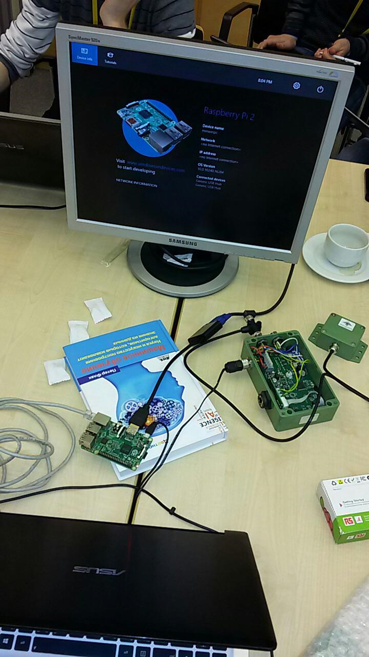
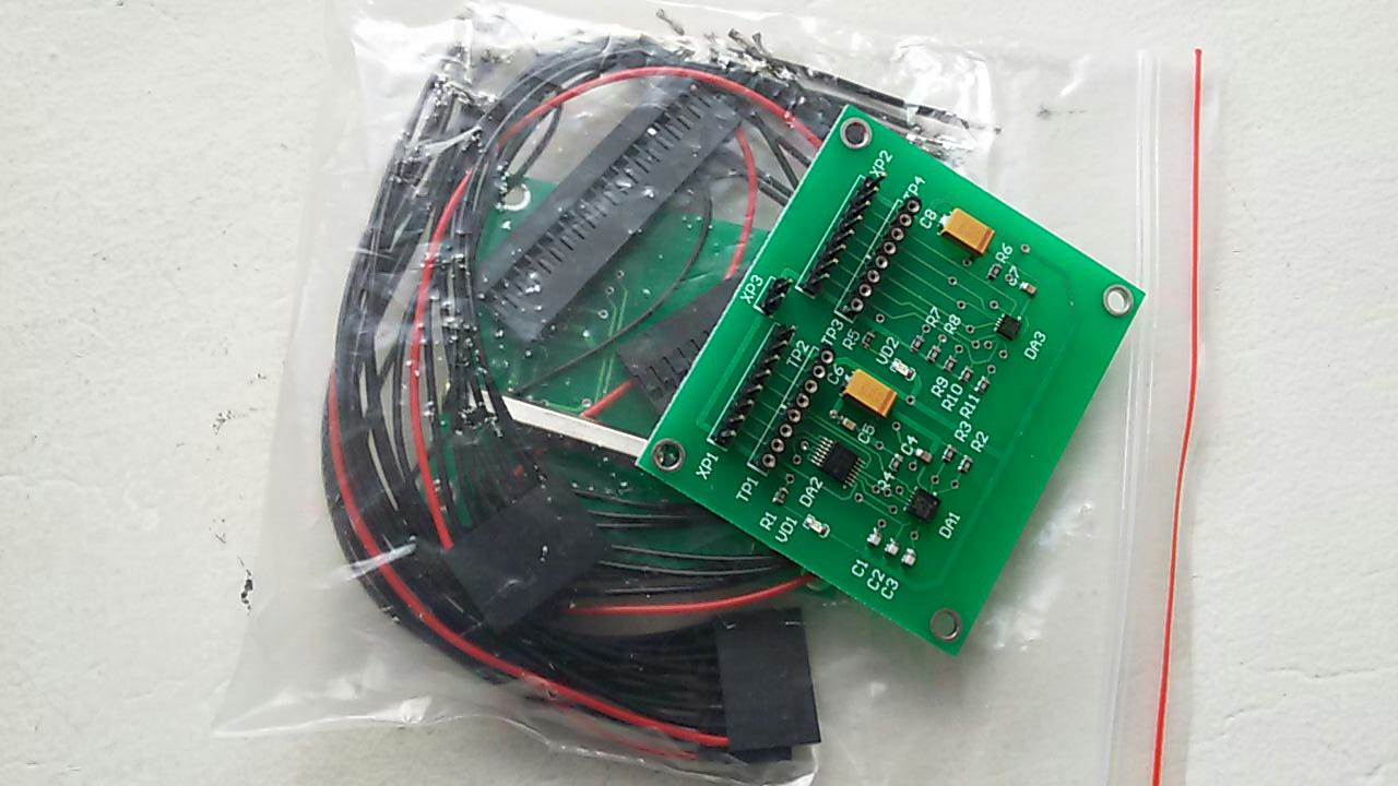
Initially, I wanted to do everything on the Raspberry Pi 2 and Windows IoT . A special board was prepared (in the photo below) with digital and analog accelerometers, but I did not manage to try it in practice, having decided to do everything on a hackathon. Just in case, I also captured our sensor , which also allows you to learn “raw” data on fluctuations.



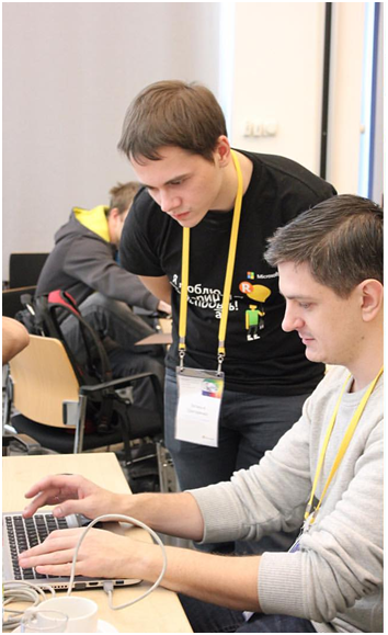
At the hackathon, all participants were asked to split into teams and solve one of 3 problems using pre-prepared data. My task turned out to be “out of competition”, but the team gathered quickly enough:



None of us had experience using Azure Machine learning, so there was a lot to do! Thanks to colleagues, among whom was psfinaki , for their efforts!

It was decided to divide into 3 directions:

• preparation of data for analysis
• upload data to the cloud
• work with Azure Machine Learning

The preparation of the data was to get it from the accelerometer, and then present it in a form available for download to the cloud. Upload to the cloud was planned through the Event Hub . Well, then you had to understand how to use this data in Azure Machine Learning.

Problems began on all three points.



It took a long time to configure Windows IoT on Raspberry. She did not give out a picture on the monitor. It was possible to solve this only by entering the following lines in config.txt:

hdmi_ignore_edid=0xa5000080
hdmi_drive=2
hdmi_group=2
hdmi_mode=16

This tuned the video driver to the desired format, resolution and frequency.



However, the time spent on this lesson made it clear that you just might not have time to organize the receipt of data from the accelerometer. Therefore, it was decided to use the sensor that I had taken in reserve.

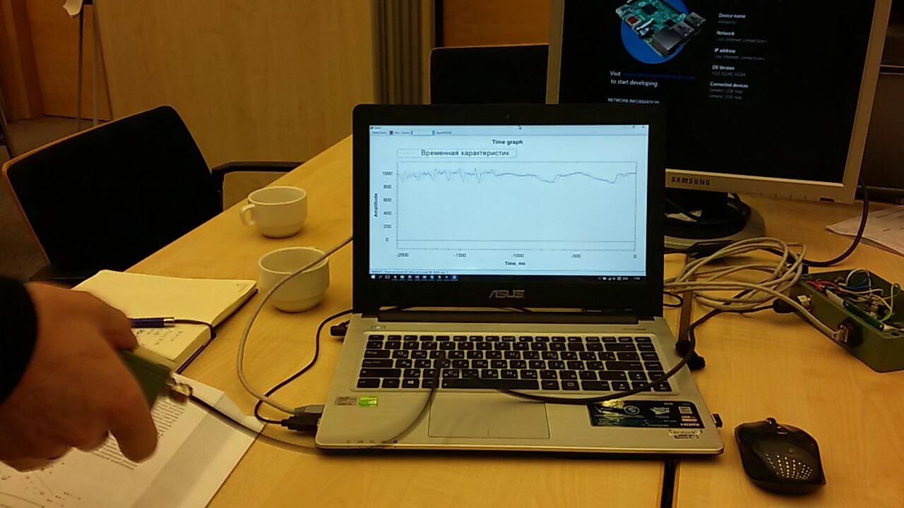
Many applications have already been written for the sensor. One of them displayed on the screen a graph of “raw” data:



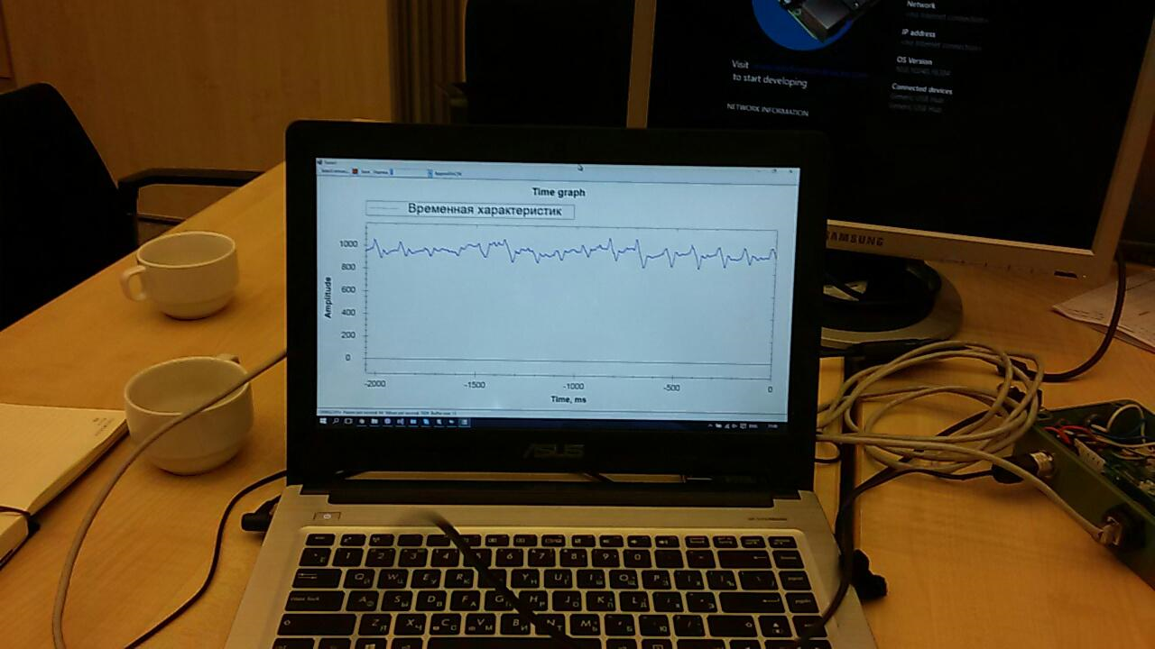
It was necessary to finish it a bit in order to prepare the data for sending to the cloud.

Event Hub also did not work right away. To begin with, we tried to send there just a random sequence. But the data did not want to appear in the reports. There were several problems, and, as it turned out, they were all “childish”: they set up something wrong, somewhere they used the wrong key, and so on. Work in this direction was difficult and took a lot of energy:



But, by the evening of the first day, we were able to send and receive data from the sensor on the fly ... True, this was not necessary in the final solution. I’ll tell you about the reasons a little later.

With Machine Learning, nothing was clear at all. At first we together studied the beautifulAn article with an example of using a mobile application as a client. Then we figured out the data format and how to work with them. Then they thought how to create training sequences.

Azure Mashine Learning has many algorithms for various classification. These algorithms must be trained on a test data set. Then, those that give the best result can be published as a web service and connected to them from the application.

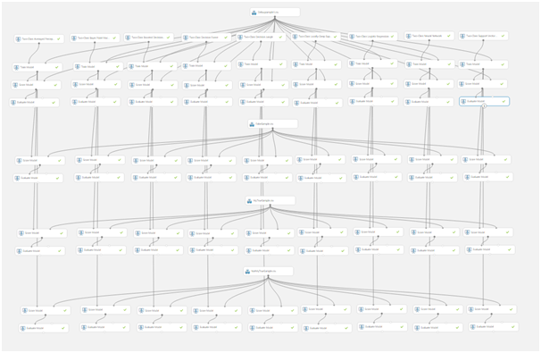
Learning an algorithm is called an “experiment." All actions are carried out in a visual editor:



Dragging and dropping items from the list on the left allows you to receive data, modify and transform them, train models and evaluate their work.

This is what a typical experiment looks like:



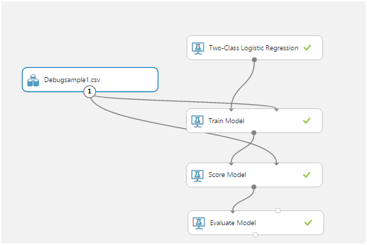
The most important were the Train Model, Score Model, and Evaluate Model.
The first, using the input data, trains the algorithm, the second tests the trained algorithm on the data set, the third evaluates the test result.

The source data in our case is a csv file. But what should be contained in it?

The sensitive element of our sensor is interrogated 1024 times per second. Each survey is a two-byte value corresponding to the amplitude of the current oscillation. Moreover, the amplitude is measured not from zero, but from the reference number corresponding to a stationary sensor.

Upon reflection, we decided to use temporary slices. For example, all sensor polls for 256 ms gave us one line in the csv table. This data, in an additional column, could be marked in one way or another, depending on what is happening with the sensor. For example, we used 0 to indicate noise (shaking the sensor with your hands, tapping, etc.) and 1 to indicate the signal (there is a vibrating telephone on the sensor).

This is how we wrote down the test sequences:



Having received the data and understanding what needs to be done with them, we began to learn the first model:



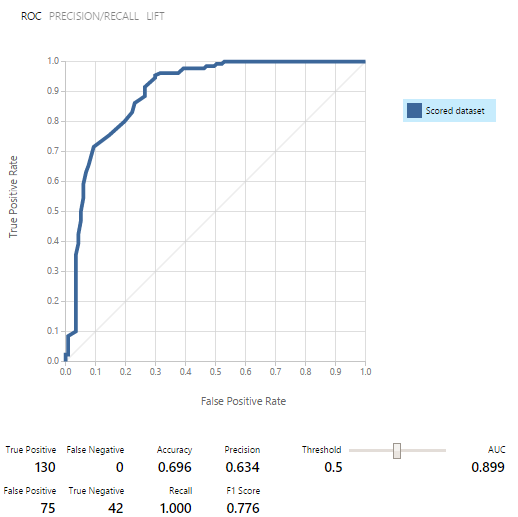
The first pancake turned out to be lumpy:



At that time, even the meaning of these indicators was not clear. We were saved by a representative of the support team, Yevgeny Grigorenko, talking about the ROC curves. The main thing was that if the graph is below the midline in some place, then the model works even worse than if it gave a random result! Eugene continued to help us as much as he could, for which many thanks to him!



Then we rewrote the training sequence for a long time and looked at the results:



It turned out that working with a 2 second recording turned out to be less optimal (2048 sensor polls). This allowed us to make table csv rows more meaningful. But the result was still far from good.

This ended the first day.

I spent the night studying the material. The article really helpedabout binary classification. I also carefully read the article with tips for this hackathon. In general, by the beginning of the work I was full of new ideas.

We spent the entire first half of the second day studying different models. The result of the work was such a “sheet”:



By this time, it was already clear that we simply did not have time to distinguish between two vibration rings, since the quality of the training data left much to be desired, and there was not enough time to record new ones. Therefore, we focused on the separation of data into “signal” and “noise”.

For work, we used 3 data sets:

1. A training kit in which there was a signal (lines of the csv file marked 1) and noise (lines marked 0)
2. A set containing only noise (lines from 0)
3. A set containing only the signal (lines from 1)

Models were first trained, then tested and evaluated on each of the data sets. The results were encouraging:



As a result, out of nine models of binary classification, we selected five.

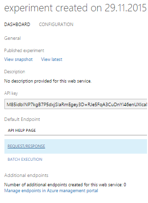
As it turned out, using the model as a Web service is much easier than screwing it to the Event hub. Therefore, we decided to publish all 5 models and work with them through REQUEST / RESPONSE, which is accompanied by a very good example.



The request is an input array of 2048 values ​​taken from the sensor. The answer looks like this:



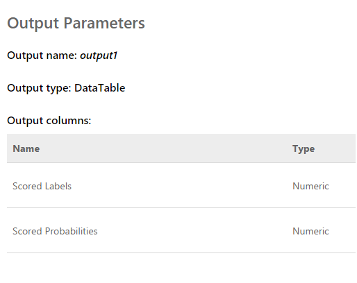
Scored labels are either 0 or 1. That is, the result of the classification. Scored Probabilities - a decimal number that reflects the correctness of the assessment. As I understand it, the first value is rounding the second. That is, the closer the second value to 0, the score 0 is more likely, and vice versa. The closer the value is to 1, the score 1 is more likely.

Having finalized the program that displays the “raw data” graph on the screen, we were able to simultaneously receive data from all five web services from several streams. Further, after observing the estimates a little, we excluded one, since it gave a result that was completely different from the others and spoiled the whole picture.

The result is the following:







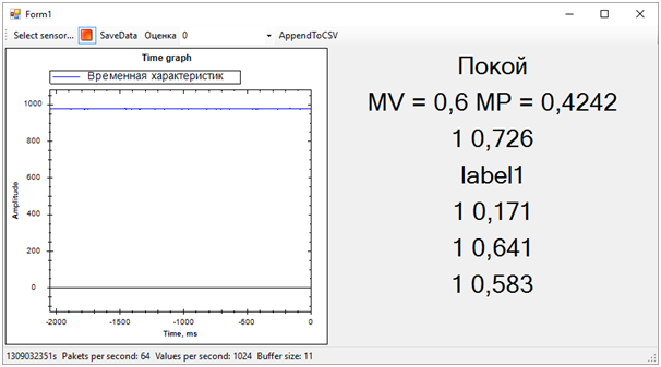
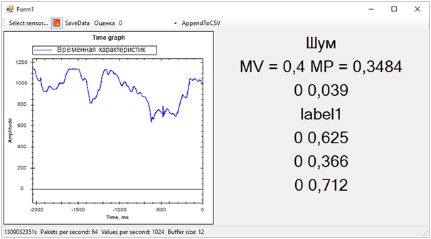
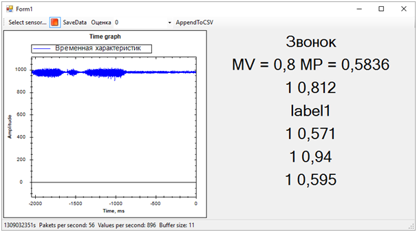
Then all the problems of the training sequence immediately got out. Although we tried to separate the vibration alert from everything else (noise and rest), the rest state turned out to be very close to the call, this was not always determined. The difference between the call and the rest, we determined by the average number of probabilities for each model. A value closer to 1 means a call, a value of about 0.5 with a score of 1 is peace. Well, if the score is 0 - this is definitely noise.

At this time, the hackathon came to an end. We didn’t even have time to show the results to the experts, as they were busy evaluating the entries.

But all this was no longer of particular importance. Most importantly, we have achieved a completely sane result and at the same time have learned a lot!

In two days of hard work, we completed, although partially, the task. Thanks to the colleagues from the team and the experts who helped us!

Now we can note the development paths of our project. We used time characteristics to separate events. However, if we move to the frequency domain, the efficiency of the algorithms should be higher. Noise, peace and bell have noticeably different spectral characteristics.

In addition, experienced people suggested that data should be normalized. That is, the numbers of the input sequence must be in the range from -1 to +1. Algorithms work more efficiently with such data.

Well and still, it is necessary to work on the formation of training sequences in order to more clearly separate the signal from noise.

These improvements should significantly increase the accuracy of state determination, which I want to check in the future.