tl; dr:

Scientists from Columbia University, led by Ken Shepard and Rafa Yuste, said they had bypassed the centennial counting theorem (Nyquist-Shannon theorem, discretization theorem, in Russian-language literature - Kotelnikov's theorem): 1 , 2 . Now, anti-aliasing filters have become optional, since noise from superimposing spectra can be restored after sampling. Sound crazy? Yes. I offer $ 1,000 to the first who proves that this is not insanity. To receive a reward, be sure to read to the end.

“Filter before sampling!”

This mantra is driven to death in the heads of generations of engineering students. Here, "discretization" refers to the conversion of a continuous function of time into a series of discrete values. Such a process occurs wherever a computer digitizes a signal from the real analog world. “Filter” means to remove high-frequency components from the signal. Since this process takes place in the analog world, it requires real analog equipment: circuits of resistors, capacitors and amplifiers. Creating such a circuit can be a tedious and time-consuming process, for example, if there is not enough space on the electronic circuits. Shepard's research team examined this limitation in the context of a device for recording signals from nerve cells .

Now, the authors claim that they have invented a “data collection paradigm that does not require filters for overlay protection for each channel, thereby overcoming the scaling limitations of existing systems.” In fact, they say that instead of hardware circuits, you can use software that works on the digital side after sampling . “Another advantage of this approach to data collection is that all steps of the signal processing (channel separation and deletion) are implemented in digital form,” the scientific work says .

If true, it would be a major discovery. It not only refutes the generally accepted opinion, which has been held for almost a century. Yeshe and a bunch of equipment is becoming unnecessary. Overlay filters are commonly used in electronic equipment. Your mobile phone has several digital radio chips and an analog-to-digital audio signal converter, and between them there are half a dozen filter microcircuits for protection against overlapping. If all of these electronic components can be replaced with a few lines of code, then manufacturers are happy to do so. So this is potentially a billion dollar idea .

Unfortunately, this is a big mistake. I will show that these documents have nothing to do with the discretization theorem. They do not cancel processing. And do not cancel analog filters before digitization. And they don’t even come close to the best systems for extracting neural signals from noise.

Why overlay is bad

[skip this part if you know the answer]

Discretization is the most important stage of data collection when a continuous signal turns into a discrete series of numbers. Most often, a continuous signal is a voltage signal. It is sampled and digitized at regular intervals by an electronic circuit called an “analog-to-digital converter” (Fig. 1). At first glance, information is lost due to sampling. Indeed, there are “infinitely many” points on a continuous voltage curve, but after sampling we leave only a part of them. Consequently, an infinite number of points between the selected ones is lost. And here the most important statement of the discretization theorem sounds :under appropriate conditions, individual samples contain all the information necessary for the ideal restoration of the continuous voltage function that produced them . In this case, there is no loss of information due to sampling.

These corresponding conditions are simple: the input signal must change slowly enough so that its shape is well fixed in the sequence of discrete samples. In particular, the signal should not have sinusoidal components at frequencies higher than the so-called Nyquist frequency, which is equal to half the sampling frequency:

$$

(1)

For example, if the ADC takes 10,000 measurements per second, then the input signal should not exceed a frequency of 5000 Hz. What happens if the input signal changes faster? These frequency components cannot be reconstructed from samples, since their origin is completely incomprehensible (Fig. 1).


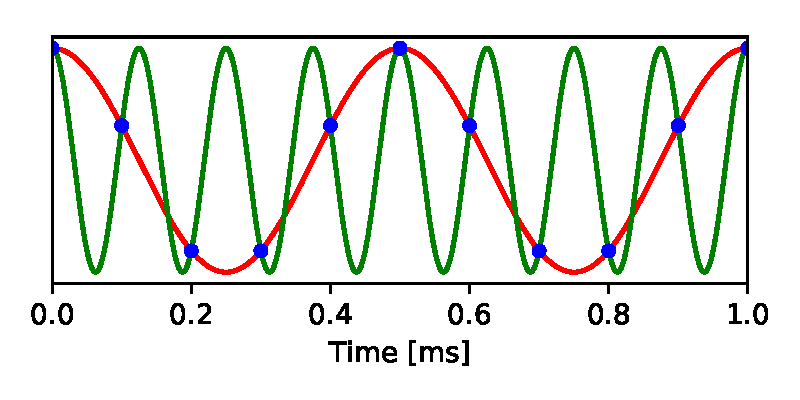
Fig. 1. Overlay. A 2 kHz sine wave (red) is sampled at 10 kS / s (blue dots). Another sine wave with a frequency of 8 kHz produces exactly the same sequence of samples. Thus, after sampling, it is impossible to understand whether the original signal was 2 kHz or 8 kHz. The

same set of samples is obtained both from a signal below the Nyquist frequency and from any number of possible signals above the Nyquist frequency. This phenomenon is called overlay (aliasing) when the high-frequency signal in sampled form may masquerade as a low frequency signal. If there are no restrictions for the incoming signal, then the overlay leads to the loss of information, because we can no longer restore the original signal from discrete samples.

How to avoid overlap? You just need to eliminate the frequency components above the Nyquist frequency from the analog signal before sampling. Most often this is done with an electronic low-pass filter that passes low frequencies but cuts off high frequencies. Thanks to the widespread use of such filters, a lot of engineering effort has been spent on improving them. As a result, the usual approach to designing a data acquisition system looks like this (Fig. 2):

1. Determine the necessary bandwidth of the signal that needs to be registered, namely the highest frequency that needs to be restored later. This is the Nyquist frequency$$for your system.

2. Pass the signal through a low-pass filter that cuts off all frequencies above$$.

3. Start sampling the signal after the filter with a frequency$$.


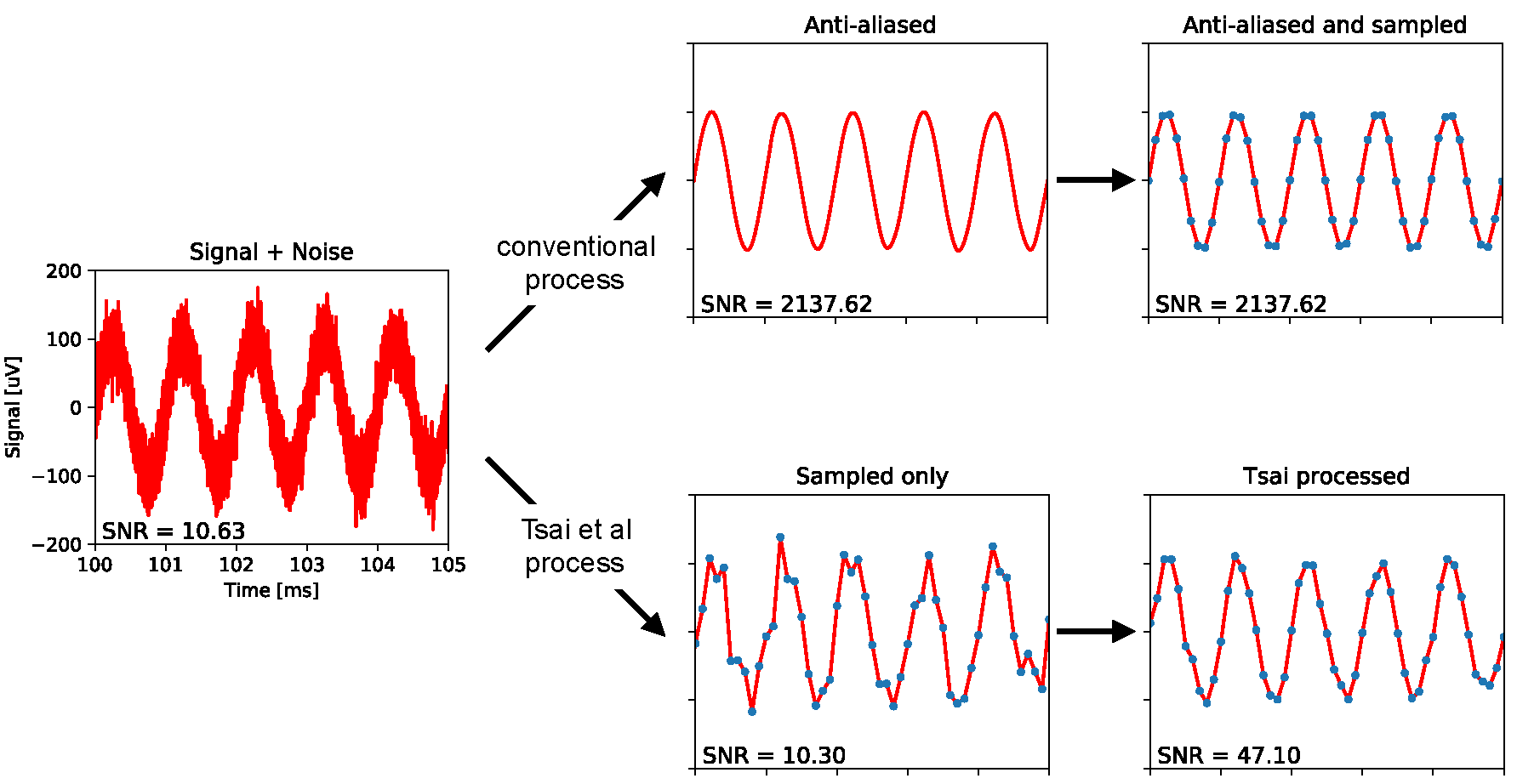
Fig. 2. Comparison of the usual data collection with the procedure described in the scientific work of Tsai et al. Left: a sine wave at a frequency of 1 kHz with an amplitude from peak to peak of 200 μV, as in test records from scientific work. Added white Gaussian noise with a bandwidth of 1 MHz and an rms amplitude of 21.7 μV. Above: a standard filtering protection approach with a cut-off frequency of 5 kHz, which eliminates most of the noise and thus improves the signal-to-noise ratio (SNR) by 200 times. This signal is then digitalized at 10 kS / s. Bottom:in the scientific work of Tsai et al., the signal is immediately sampled while maintaining the same low SNR. This is followed by digital processing, which slightly increases the SNR. All data and processing are modeled using this code.

What Tsai et al claim

Now consider a specific situation from the scientific work of David Tsai et al. They want to record electrical signals from neurons, which requires a bandwidth

$$

So they chose a sampling rate of 10 kS / s. Unfortunately, the required neural signal is distorted due to wideband thermal noise, an inevitable by-product during recording. The noise spectrum reaches 1 MHz with a typical rms amplitude (rms) of 21.7 μV. The authors approximate it as white Gaussian noise, that is, noise with a constant power density up to a cutoff of 1 MHz. (References to these figures: p. 5 and Fig. 11 from the first article ; p. 2, 5, 9 and Fig. 2e in the appendix from the second article ).

The standard procedure would be to transmit signal and noise through an analog filter to protect against overlapping with cutoff frequencies above 5 kHz (Fig. 2). This will leave the neural signal intact, while at the same time reducing the noise power by 200 times, because the noise spectrum is cut from a 1 MHz bandwidth to only 5 kHz. Thus, the remaining noise below the Nyquist frequency will have a rms amplitude of only 21.7 μV /$$ = 1.53 μV. Such an amount of thermal noise is completely harmless. This is less than from other sources of noise in the experiment. The signal is then sampled at a sampling rate of 10 kS / s.

Instead, the authors completely exclude the filter and directly sample the broadband signal + noise . In his articlethey explain in detail the technical limitations associated with the lack of space on silicon devices in this recording method, because of which it was necessary to abandon the filter. But in the end, all the noise power up to 1 MHz has now hit the sampled signal through overlay. In fact, each sample is contaminated with Gaussian noise with a rms amplitude of 21.7 μV. This is an unacceptable noise level because we want to distinguish between neuron signals at the same or lesser amplitude. For reference, in some popular systems for recording multi-neural activity, the noise level does not exceed 4 μV.

Here Tsai and his colleagues demonstrate amazing “innovation”: they say that it’s possibleapply a cunning algorithm of data conversion after sampling to restore the original broadband noise , subtract this noise from the sampled data - and thus leave a clean signal. Here are the relevant quotes, in addition to the above: “We can digitally reconstruct the spectral contribution from high-frequency thermal noise, and then remove it from the data with sparse sampling, thereby minimizing the effects of overlap, without using anti-aliasing filters on each channel.” And one more: “We present multiplexing architectures without overlay filters on each channel. Sparse data are recovered using a compressed readout strategy that includes statistical reconstruction and removal of thermal noise with a coarse sampling step. ”

What evidence do they provide for this statement? Only one experiment was conducted that checks noise reduction using real data. The authors recorded a sinusoidal test signal at a frequency of 1 kHz with an amplitude of 200 μV from peak to peak. Then they applied their processing scheme to “remove thermal noise”. The output signal looks cleaner than the input (Fig. 2e from the article; see also the simulation in fig. 2). Quantitatively, the noise was reduced from a rms amplitude of 21.7 μV to 10.02 μV. This is a rather modest improvement in signal-to-noise ratio (SNR) by 4.7 times (more on this below). A proper anti-aliasing filter before sampling, or a declared superimposed noise removal system after sampling, should increase the SNR 200 times. (For links to the cited results, see Fig. 2e-f from the second article and Fig. 7 from the first article ).

Why the scheme of Tsai et al. Cannot work in principle

Before proceeding to a specific analysis of the data processing scheme proposed in these scientific articles, it is worth considering why it cannot work in principle. The most important thing: if it works, then this cancels the Kotelnikov theorem, which generations of engineering students studied at institutes. The white noise signal in these experiments is sampled at a frequency 200 times lower than that which allows us to reconstruct this signal using the Kotelnikov theorem. So why did Tsai and colleagues decide that the circuit could work?

The authors claim that the superimposed high-frequency noise preserves a certain imprint, which allows you to remove it: “Using the above characteristics, we can digitally restore the spectral contribution from high-frequency thermal noise, and then remove it from the data with sparse sampling, thereby minimizing the effects overlay ". It is difficult to understand what these characteristics may be. They are easiest to evaluate on a timeline. White Gaussian noise in the 1 MHz band can be reconstructed from the time series of independent samples from an identical Gaussian distribution with a frequency of 2 million samples per second. Now take these time series and make a subsample of 10 thousand samples per second, i.e. every 200th of the original samples. You will again receive independently and equally distributed samples, i.e. white Gaussian noise at 10 kS / s. Nothing in this series of samples shows that its source is high-frequency noise. It is well discretized.


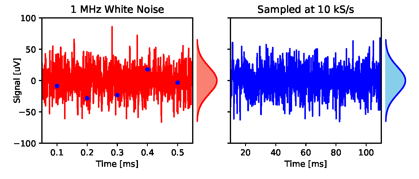
Fig. 3. A sample of white Gaussian noise. Left: white Gaussian noise (red line) with a rms amplitude of 21.7 μV and a bandwidth of 1 MHz is sampled at a frequency of 10 kS / s (blue dots). Right: discretized signal with 200 times extended timeline. This is also white Gaussian noise, with the same amplitude distribution (graph field), but with a bandwidth of 5 kHz

The authors also argue that their algorithm for reconstructing white Gaussian noise “avoids overlapping through the use of compressed read concepts”. The principle of compressed sensing is that if a signal exhibits known patterns, then it can be discretized without loss with a frequency less than the Nyquist frequency. In particular, such a signal exhibits a rarefied distribution in the data space in certain directions, which opens up possibilities for compression. This applies to many natural sources of signal, such as photographs. Unfortunately, white Gaussian noise is an absolutely incompressible signal without any patterns. The probability distribution for this signal is a round Gaussian sphere, which in the data space looks the same from all sides and simply does not provide any compression capabilities. Of course, neural signals on top of this noise contain some statistical patterns (more on this below). But they do not help restore noise.

How the scheme of Tsai et al. Fails in practice

I wrote the code for the algorithm described in the scientific work of Tsai et al. When processing the simulation of the author’s test (a sinusoidal wave of 200 μV with a noise of 21.7 μV), it produces a purified sinusoidal wave with a noise of only 10.2 μV (Fig. 2), which terribly close to the result from scientific work of 10.02 μV. So, I correctly emulated the circuit.

Along the way, I came across something similar to a serious mathematical error. This refers to the authors' belief that noise with insufficient sampling steps retains a certain signature as a result of overlapping. Referring to the Fourier representation of white Gaussian noise, they write ( section III.G): “In the Fourier space, the vector angles of thermal noise (infinite length) have a uniform distribution with zero mean. Again, any deviation from this ideal in finite-length signals is averaged by overlapping spectra when the content is added to the first Nyquist zone (as a result of which the angles converge to zero). " And similarly, “spectral angles converge to zero in the variant of superimposing thermal noise” ( page 9, bottom left) This is not true. The phase angles of the Fourier vectors described here have a uniform circular distribution; this distribution does not have an average angle. After averaging due to the normalization of some of these vectors, the phase of the average vector again acquires a uniform circular distribution. This is confirmed in Fourier space, which is easier to estimate in direct space: a subsample of white Gaussian noise again gives you white Gaussian noise (Fig. 3). The rationale for Tsai's algorithm is based on this erroneous concept that the phase angles are somehow averaged to zero.

So, how does the Tsai algorithm clear a sinusoidal test signal? This is not so difficult. If you know that the signal is a pure sine wave, then only three unknowns remain: amplitude, phase and frequency. Obviously, you can extract these three unknowns from the 10,000 noise samples that you get every second. It can be done much more efficiently: find the largest Fourier component in the sampled record and zero out all the others. This almost completely eliminates noise (see here for details ). Tsai’s algorithm does something like this: it suppresses off-peak frequencies in the Fourier transform more strongly than peak ones and receives a certain sum of a sinusoid and suppressed noise (see also Fig. 9 in the work ). As we will see later, the claimed performance does not apply to realistic signals.

What would be a reasonable processing scheme?

The sine wave example shows how you should actually approach data postprocessing. An attempt to restore the original noise is hopeless for all the reasons described above - you just need to put up with the noise level that is the result of all overlapping spectra. And focus on the properties of the signal that we want to highlight. If the signal has statistical patterns, then this fact can be used to your advantage. Naturally, a sine wave is extremely regular - which means that it is extracted from the noise with almost infinite accuracy. Usually we have some partial knowledge of signal statistics. For example, the shape of the energy spectrum. Neural action potentials have frequency components up to ~ 5 kHz, but the spectrum is not flat in the entire range (Fig. 4).


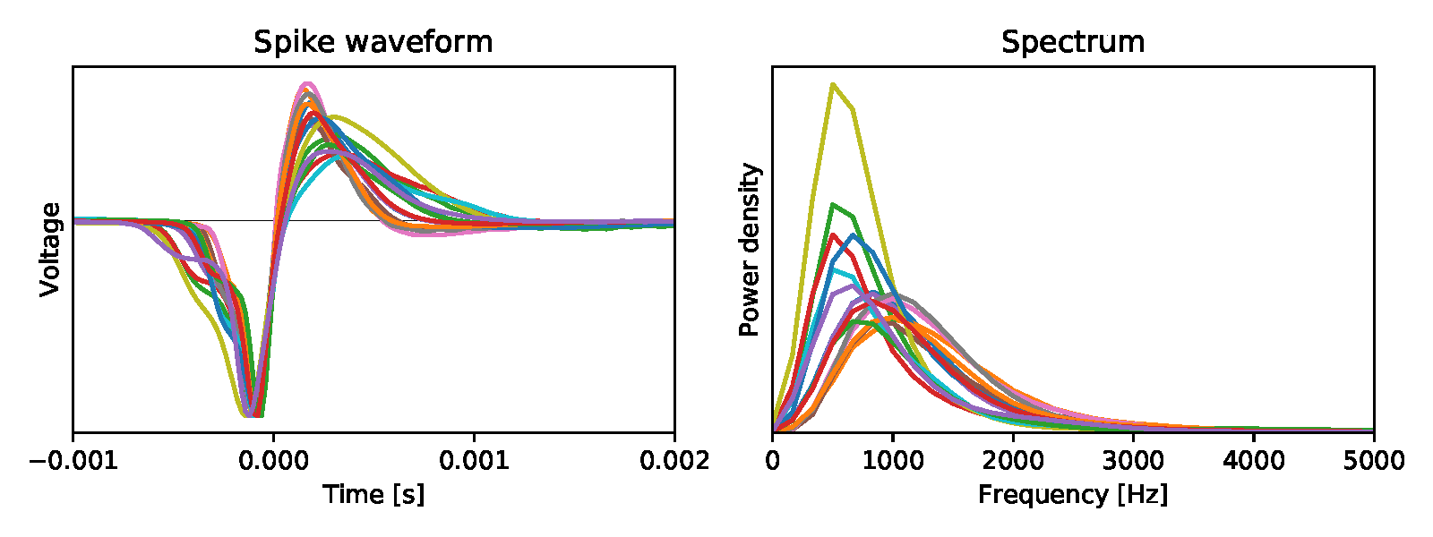
Fig. 4. Left:averaged bioelectric potentials for 15 mouse retinal ganglion cells [ source ]. Right: their energy spectrum.

Suppose we know the energy spectrum of a signal, and it differs from the noise spectrum — how then to process the sample data in order to optimally recover the signal? This is a classic task that is asked on the signal processing course. The optimal linear filter for reconstruction with minimization of the mean square error is called the Wiener filter . In fact, it suppresses frequency components where the noise is relatively larger. But Tsai’s algorithm is a non-linear operation (see details here), so theoretically it can surpass the Wiener filter. In addition, due to non-linearity, it is impossible to predict the efficiency of an algorithm on more ordinary signals by its performance on sinusoidal signals (see above). Therefore, I compared the Tsai algorithm with the classic Wiener filter, using various assumptions for the spectrum. In particular, the signal was limited below the cutoff frequency in the range from 100 Hz to 5000 Hz, while the noise had a uniform spectrum in the 5 kHz band:


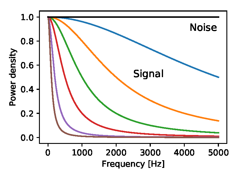
Fig. 5. The energy spectrum of the signal (colored lines) and noise (black) used in the calculations in Fig. 6. Gaussian noise and white throughout the range. The signal is obtained from a Gaussian white process passed through a single-pole low-pass filter with cutoff frequencies at 5000, 2000, 1000, 500, 200, 100 Hz.

For each of these combinations of signal and noise, I applied the Wiener filter and Tsai's algorithm - and measured the signal-to-noise ratio (SNR) as a result (Fig. 6).


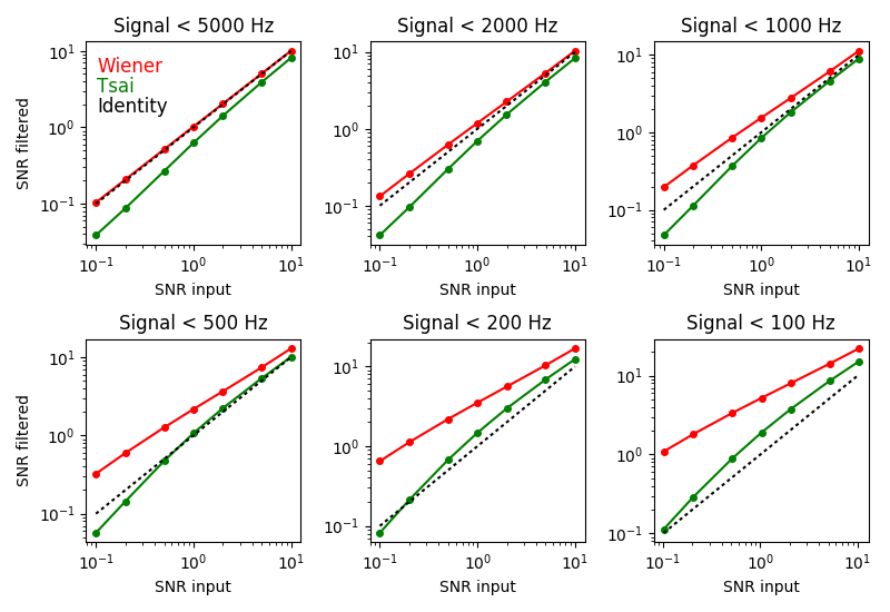
Fig. 6.How the Tsai algorithm and the Wiener filter change the SNR. Each panel corresponds to a different energy spectrum of the signal (see Fig. 5). The signal and noise on different SNRs are plotted along the horizontal axis. The mixed signal and noise were passed through a Wiener filter or Tsai algorithm, and the SNR of the output signal is plotted along the vertical axis. Red - Wiener filter; green - Tsai algorithm; the dotted line is the original.

As expected, the Wiener filter always improves the SNR (compare the red curve with the dotted script), and the greater the greater the difference between the signal and noise spectra (panels from upper left to lower right). In all cases, the Wiener filter surpasses Tsai's algorithm in improving SNR (compare red and green curves). In addition, in many cases, the Tsai algorithm actually worsensSNR (compare green and dashed curves). Given that the algorithm is based on mathematical errors, this is not surprising.

There are more sophisticated noise reduction schemes than the Wiener filter. For example, we know that the recordings of neural activity of interest are an imposition of pulse-like events - bioelectric potentials - whose waveforms are described by just a few parameters. Within the framework of this statistical model, it is possible to develop algorithms that determine the optimal peak values ​​of each event among noise. This is an active area of scientific research .

Why is it important for neuroscience

Researchers from various neurosciences are actively seeking to increase the number of simultaneously tracked neurons. In this area, exponential progress, although rather slow, is doubling every seven years . Several projects are aimed at accelerating this process by creating large-scale CMOS chips with an array of thousands of densely arranged electrodes and multiplexers [including Tsai's work - note. trans.]. This is expensive research. To bring the electrode arrays to the prototype stage, millions of investments are required. If the success of such a device is based on erroneous notions of overlap and unjustified expectations from software, this can lead to costly failures and waste of valuable resources.

The Fromherz massif became a painful failure of this kind . Designed in collaboration with Siemens for millions of Deutschmarks, it has become the largest array of bioelectrodes of its time, with 16,384 sensors at a site of 7.8 × 7.8 microns. To save space and for other reasons, developers have refused to use anti-aliasing filters. Overlay and other artifacts eventually led to a noise level of 250 μV , unsuitable for any interesting experiments, so the innovative device was never used in practice. But such an outcome could be predicted by a simple calculation.

If it is rational to foresee the consequences of overlapping, then useful trade-offs are possible. For example, in a newly created device with silicon pinsthere are also no anti-aliasing filters in multiplexers . But the coefficient of subsampling is only 8: 1, as a result of which the excess noise does not exceed critical values . In combination with proper signal recovery, such a circuit is quite viable.

Who checked this work?

As always, the question arises: did these dramatic statements by Tsai et al. Be reviewed? Was anyone really surprised by the apparent contradiction of the counting theorem? Who reviewed these materials at all? Well, I reviewed them. For another magazine, where the article was eventually rejected. Prior to this, there was a lengthy correspondence with the authors, including I gave them the task of removing the overlay noise from the simulated record (task below, only without a monetary reward). The authors considered the challenge a reasonable test of the algorithm, but failed the test completely. Somehow, this did not shake their confidence - and they submitted the exact same scientific article to two other journals. These journals, apparently after the so-called peer-review, gladly agreed to print.

How to win $ 1000

Of course, there is a chance that I misunderstood Tsai's algorithm or, in spite of everything, there is another scheme for recovering superimposed white noise after sampling. To encourage creative work in this area, I propose the task: if you can do what Tsai and his colleagues say, I will give you $ 1000. Here's how it works:

First you send me $ 10 for “postage” (Paypal meister4@mac.com, thanks). In return, I send a data file containing the result of sampling the signal and noise by 10 kS / s, where the signal is limited to a band below the Nyquist frequency of 5 kHz, and the noise is white Gaussian noise with a band of 1 MHz. You use the Tsai algorithm or any other scheme of your choice to remove the superimposed noise as much as possible, and send me a file with your best signal estimate. If you can improve your SNR two or more times, I will pay you $ 1,000. Please note that the correct anti-aliasing filter increases SNR by 200 times (Fig. 2), and Tsai claims that it increases by more than four times, so I ask a little here. For more technical information, see the code and comments in my Jupyter notebook .

A few more rules: the offer is valid for 30 days from the date of publication [March 20, 2018 - note. trans.]. Only the first qualifying record wins. You must uncover the algorithm used so that I can reproduce its work. After the battle with the sampling theorem, you may be interested in some other task, for example, a cryptographic attack on a random seed, which I used to create a data file. Although I would be interested to know about such alternative solutions, but I will not pay $ 1000 for this, but only return your $ 10.

Finally, I do not want to take money from beginners. Before you send me $ 10, be sure to carefully test your algorithm using the code in my Jupyter notebook : I will use it to evaluate the algorithm.

Summary

So far, no one has received $ 1,000, the conclusions are as follows:

• Tsai and colleagues developed a digital converter without an overlay protection filter, resulting in approximately 200 times more noise from thermal fluctuations than could be expected.
• Their post-processing algorithm does nothing to offset the effect of blending. At best, this is an attempt to separate the desired signal from the distorting superimposed noise. Unfortunately, the algorithm is based on mathematical errors.
• The best algorithms for separating a signal from white noise are well known. For sinusoidal signals (as given by the authors), such a separation is trivial. For band-limited signals whose spectral power is different from the noise spectral power, the classic solution is the Wiener filter. Under all the conditions tested, it shows a better result than the Tsai algorithm. Under many conditions, the Tsai algorithm degrades the signal-to-noise ratio.
• At the moment, I propose that hardware developers stick to the ancient wisdom of “filter before sampling!”