The basics of quantum computing: pure and mixed states
- Transfer
Recently, we talked about a way to visualize one-qubit states — the Bloch sphere. All pure states correspond to points on the surface of the Bloch sphere, and mixed states correspond to points inside it. In this publication, we will try to explain what pure and mixed states actually are.

A rigorous mathematical explanation is given in the book by M. Nielsen I. Chang, “Quantum Information and Quantum Computing,” in Section 2.4.1: “Ensembles of Quantum States,” as well as in these remarkable summaries (and in the corresponding lecture notes) of Professor Leonard Suskind of Stanford University.
A pure state is a state that can be represented by a single state vector | ψι〉. From a practical point of view, this means that at any moment in time we accurately (with a probability of 100%) know that our system is in the state | ψι〉. In other words, if the system is in a pure state, we have a complete picture of it and we know exactly what state it is in.
Examples of pure states: | 0>, | 1>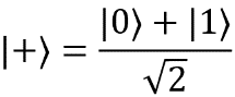 ,
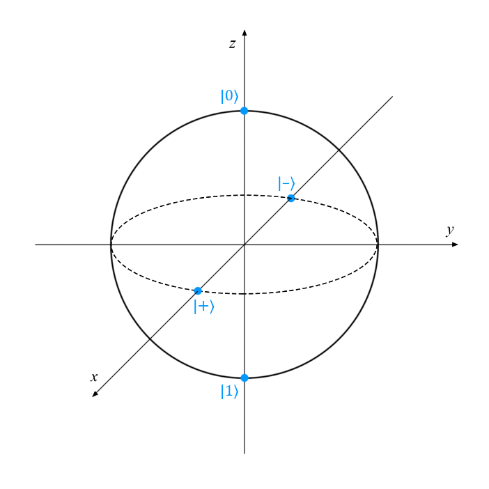
, 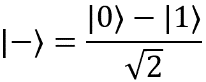 . The following points on the surface of the Bloch sphere correspond to them:
If there is no complete idea of the state in which the prepared system is, then they say that it is in a mixed state. This situation can be caused by many reasons: for example, incorrect setup of laboratory equipment or confusion of particles with an external system that is not available to us. However, if the system is in a mixed state, we cannot be 100% sure whether it is in a clean state or
or  in any other possible state. In this case, the state of the system is described by the probabilistic distribution of all pure states in which it can be with non-zero probability after preparation.
Consider an example. Let's say our colleague Mary prepared qubits for our experiment. She tries to sabotage the work and does not tell us what state each qubit is in, but we know that there are only three possible options: these are pure states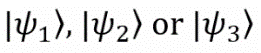 . Therefore, our initial state must be described in the language of probability theory
 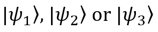 . This combination of pure states is called a mixed state.
Let us know that Mary (for example) prepares a fortunetwice as often as or . We can use this knowledge to describe the probabilities of the possible states of our system at the beginning of the experiment. If we do not know exactly how Mary chooses the prepared states, then we should assume that they are all equally probable. And now it's time to talk about the density matrix (or density operator).
The density operator (ρ) can be used to represent the state of a system whose initial state is not known for sure. This operator is a generalization of state vectors (which are used to record pure states). The density matrix for a pure state naturally degenerates into the state vector | ψι〉. For those who are interested, below are some mathematical calculations.
NOTE. It is assumed that the reader owns the basic concepts of vector and matrix algebra: external and internal product, orthogonality, etc. To get acquainted with them, it is recommended to refer to the book by M. Nielsen and I. Chang or to the Stanford lectures, which are mentioned at the beginning of the article.
The density operator can be defined as
Here :
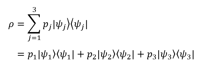
In our example, the density operator is expanded as follows:
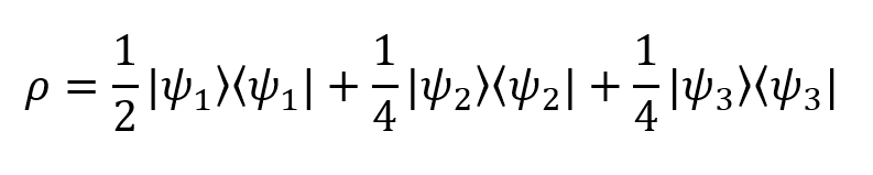
If we substitute the probability values from the above example, we get
This is the density matrix of our imaginary system! Not so difficult.
After we have calculated the density operator, it is very simple to find the probability that the measurement ρ shows some pure quantum state | ψ〉: it is equal to 〈ψ | ρ | ψ〉.
In the event that the state is pure (that is, initially the system can only be in one state), the following equality holds:
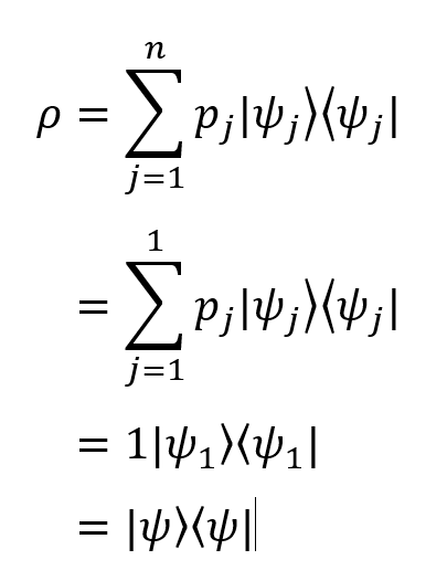
So we get the second, equivalent definition of a pure state: a state in which ρ = | ψ〉 〈ψ | (that is, with a density matrix consisting of a single projector) is clean.
We apply the density operator to our pure state vector:
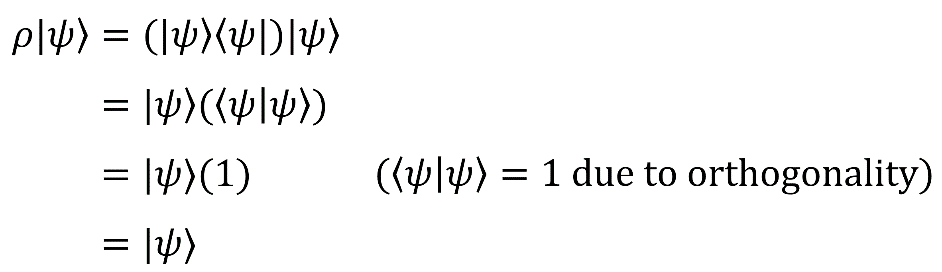
As you can see, the result is only | ψ〉.
By analogy, the probability of detecting a system in a certain state | φ〉 is equal to P = 〈φ | ρ | φ〉 = | 〈φ | ψ〉 | ².
As we see, the rules for calculating probabilities for mixed states come down to the rules for pure states that we already know. Thus, all the rules for mixed states are expressed through the rules for pure states, as previously stated.
Articles from the cycle:
A rigorous mathematical explanation is given in the book by M. Nielsen I. Chang, “Quantum Information and Quantum Computing,” in Section 2.4.1: “Ensembles of Quantum States,” as well as in these remarkable summaries (and in the corresponding lecture notes) of Professor Leonard Suskind of Stanford University.
Clean conditions
A pure state is a state that can be represented by a single state vector | ψι〉. From a practical point of view, this means that at any moment in time we accurately (with a probability of 100%) know that our system is in the state | ψι〉. In other words, if the system is in a pure state, we have a complete picture of it and we know exactly what state it is in.
Examples of pure states: | 0>, | 1>
, . The following points on the surface of the Bloch sphere correspond to them:Mixed states
If there is no complete idea of the state in which the prepared system is, then they say that it is in a mixed state. This situation can be caused by many reasons: for example, incorrect setup of laboratory equipment or confusion of particles with an external system that is not available to us. However, if the system is in a mixed state, we cannot be 100% sure whether it is in a clean state
Consider an example. Let's say our colleague Mary prepared qubits for our experiment. She tries to sabotage the work and does not tell us what state each qubit is in, but we know that there are only three possible options: these are pure states
. Therefore, our initial state must be described in the language of probability theory . This combination of pure states is called a mixed state. Let us know that Mary (for example) prepares a fortune
Density operator, ρ
The density operator (ρ) can be used to represent the state of a system whose initial state is not known for sure. This operator is a generalization of state vectors (which are used to record pure states). The density matrix for a pure state naturally degenerates into the state vector | ψι〉. For those who are interested, below are some mathematical calculations.
A bit of math
NOTE. It is assumed that the reader owns the basic concepts of vector and matrix algebra: external and internal product, orthogonality, etc. To get acquainted with them, it is recommended to refer to the book by M. Nielsen and I. Chang or to the Stanford lectures, which are mentioned at the beginning of the article.
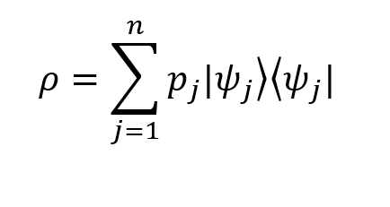
The density operator can be defined as
Here :
 - the probability that the system is in a state at the initial moment of time
  .
.- The element
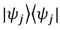 corresponds to the result of the external product of the vector
  by itself (such a transformation is also called the projection operator).
 - n is the total number of possible states of the system (in our example there are three of them).
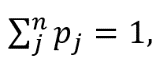 as expected (the sum of the probabilities of all possible states is 1).
In our example, the density operator is expanded as follows:
If we substitute the probability values from the above example, we get
This is the density matrix of our imaginary system! Not so difficult.
After we have calculated the density operator, it is very simple to find the probability that the measurement ρ shows some pure quantum state | ψ〉: it is equal to 〈ψ | ρ | ψ〉.
In the event that the state is pure (that is, initially the system can only be in one state), the following equality holds:
So we get the second, equivalent definition of a pure state: a state in which ρ = | ψ〉 〈ψ | (that is, with a density matrix consisting of a single projector) is clean.
We apply the density operator to our pure state vector:
As you can see, the result is only | ψ〉.
By analogy, the probability of detecting a system in a certain state | φ〉 is equal to P = 〈φ | ρ | φ〉 = | 〈φ | ψ〉 | ².
As we see, the rules for calculating probabilities for mixed states come down to the rules for pure states that we already know. Thus, all the rules for mixed states are expressed through the rules for pure states, as previously stated.