About probabilities
- Tutorial
( source )
Sometimes I have to tell other people how machine learning works, and in particular, neural networks. Usually I start with gradient descent and linear regression, gradually moving to multi-layer perceptrons, auto-encoders and convolution networks. All knowingly nod their heads, but at some point, a shrewd one necessarily asks:
And why is it so important that the variables in linear regression are independent?
or
And why are convolutional networks used for images, and not ordinary fully connected ones?
“Oh, it's easy,” I want to answer. - "because if the variables were dependent, then we would have to model the conditional probability distribution between them" or "because in a small local area it is much easier to learn the joint distribution of pixels." But here's the problem: my students still don’t know anything about probability distributions and random variables, so I have to get out in other ways, explaining more difficult, but with fewer concepts and terms. And what to do if they ask me to tell you about normalization or generative models about the batch, so I won’t know at all.
So let's not torment ourselves and others and just remember the basic concepts of probability theory.
Random variables
Imagine that we have profiles of people where their age, height, gender and number of children are indicated:
| age | height | gender | children |
|---|---|---|---|
| 32 | 175 | one | 2 |
| 28 | 180 | one | one |
| 17 | 164 | 0 | 0 |
| ... | ... | .... | .... |
Each line in such a table is an object. Each cell is the value of a variable characterizing this object. For example, the first person is 32 years old and the second is 180 cm tall. But what if we want to describe some variable at once for all our objects, i.e. take the whole column? In this case, we will have not one specific value, but several at once, each with its own frequency of occurrence. The list of possible values + the corresponding probability is called a random variable (random variable, rv).
Discrete and continuous random variables
To keep this in my head, I repeat once again: a random variable is completely determined by the probability distribution of its values. There are 2 main types of random variables: discrete and continuous.
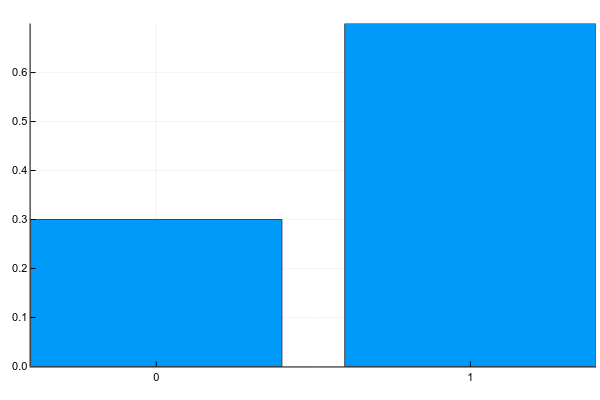
Discrete variables can take a set of clearly separable values. Usually I portray them something like this (probability mass function, pmf):
Pkg.add("Plots")
using Plots
plotly()
plot(["0","1"], [0.3, 0.7], linetype=:bar, legend=false)
And in text this is usually written like this (g - gender):
p ( g = 0 ) = 0.3p ( g = 1 ) = 0.7
Those. the probability that a random person from our sample will turn out to be a woman (g = 0 ) is 0.3, and the man (g = 1 ) - 0.7, which is equivalent to the fact that 30% of women and 70% of men were in the sample.
Discrete variables include the number of children per person, the frequency of occurrence of words in the text, the number of times a movie has been watched, etc. The result of classification into a finite number of classes, by the way, is also a discrete random variable.
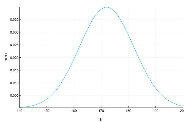
Continuous variables can take any value in a certain interval. For example, even if we record that a person’s height is 175cm, i.e. round to 1 centimeter, in fact it can be 175.8231 cm. Continuous variables are usually depicted using a probability density function (pdf) curve:
Pkg.add("Distributions")
using Distributions
xs = 140:0.1:200
ys = [pdf(Normal(172, 10), x) for x in xs]
plot(xs, ys; xlabel="h", ylabel="p(h)", legend=false, show=true)
The graph of probability density is a tricky thing: unlike the graph of probability mass for discrete variables, where the height of each column directly shows the probability of getting such a value, the probability density shows the relative amount of probability around a certain point. In this case, the probability itself can be calculated only for the interval. For example, in this example, the probability that a randomly taken person from our sample will have a height from 160 to 170 cm is approximately 0.3.
d = Normal(172, 10)
prob = cdf(d, 170) - cdf(d, 160)
Question: can the probability density at some point be greater than unity? The answer is yes, of course, the main thing is that the total area under the graph (or, mathematically speaking, the probability density integral) is equal to one.
Another difficulty with continuous variables is that their probability density is not always possible to describe nicely. For discrete variables, we just had a table of value -> probability. For continuous, this will not work, because they generally have an infinite number of meanings. Therefore, they usually try to approximate the data set by some well-studied parametric distribution. For example, the graph above is an example of the so-called. normal distribution. The probability density for it is given by the formula:
p ( x ) = 1√2 π σ 2 e-(x-μ)22 σ 2
Where μ (expectation mean) andσ 2 (variance) - distribution parameters. Those. having only 2 numbers, we can fully describe the distribution, calculate its probability density at any point or the total probability between the two values. Unfortunately, far from any data set there is a distribution that can beautifully describe it. There are many ways to deal with this (take at least amixture of normal distributions), but this is a completely different topic.
Other examples of continuous distribution: a person’s age, the intensity of a pixel in an image, response time from a server, etc.
Joint, marginal and conditional distributions
Usually we consider the properties of an object not one at a time, but in combination with others, and here the concept of joint distribution of several variables appears . For two discrete variables, we can depict it in the form of a table (g - gender, c - # of children):
| c = 0 | c = 1 | c = 2 | |
|---|---|---|---|
| g = 0 | 0.1 | 0.1 | 0.1 |
| g = 1 | 0.2 | 0.4 | 0.1 |
According to this distribution, the probability of meeting a woman with 2 children in our dataset is p ( g = 0 , c = 2 ) = 0.1 , and a childless man -p ( g = 1 , c = 0 ) = 0.2 .
For two continuous variables, for example, height and age, we again have to define an analytic distribution function p ( h , a ) , approximating it,
for example, bymultidimensional normal. You cannot write this in a table, but you can draw:
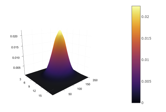
d = MvNormal([172.0, 30.0], [100; 0 5])
xs = 160:0.1:180
ys = 22:1:38
zs = [pdf(d, [x, y]) for x in xs, y in ys]
surface(zs)
Having a joint distribution, we can find the distribution of each variable individually by simply summing (in the case of discrete) or integrating (in the case of continuous) the remaining variables:
p ( g ) = ∑ c p ( g , c )p ( h ) = ∫ p ( a , h ) d a
This can be represented as a summation over each row or column of the table and putting the result in the fields of the table:
| c = 0 | c = 1 | c = 2 | ||
|---|---|---|---|---|
| g = 0 | 0.1 | 0.1 | 0.1 | 0.3 |
| g = 1 | 0.2 | 0.4 | 0.1 | 0.7 |
So we get again p ( g = 0 ) = 0.3 andp ( g = 1 ) = 0.7 . The process of submission to the field (margin) gives the name and to obtain the distribution -marginal(marginal probability).
But what if we already know the value of one of the variables? For example, we see that we have a man in front of us and want to get the probability distribution of the number of his children? The joint probability table will help us here as well: since we already know for sure that we have a man in front of him, i.e.g = 1 , we can discard all other options from consideration and consider only one line:
| c = 0 | c = 1 | c = 2 | |
|---|---|---|---|
| g = 1 | 0.2 | 0.4 | 0.1 |
ˉ p (c=0|g=1)=0.2ˉ p (c=1|g=1)=0.4ˉ p (c=2|g=1)=0.1
Since the probabilities must somehow be summed into one, the resulting values need to be normalized, after which it will turn out:
p ( c = 0 | g = 1 ) = 0.29p ( c = 1 | g = 1 ) = 0.57p ( c = 2 | g = 1 ) = 0.14
Distribution of one variable with a known value of the other is called the conditional (conditional probability).
Chain rule
And all these probabilities are connected by one simple formula called the chain rule (chain rule, not to be confused with the chain rule in differentiation):
p ( x , y ) = p ( y | x ) p ( x )
This formula is symmetrical, so this can also be done:
p ( x , y ) = p ( x | y ) p ( y )
The interpretation of the rule is very simple: if p ( x ) is the probability that I will go to the red light, andp ( y | x ) is the probability that a person switching to the red light will be hit, then the joint probability of going to the red light and being hit is exactly equal to the product of the probabilities of these two events. But generally, go green.
Dependent and Independent Variables
As already mentioned, if we have a joint distribution table, then we know everything about the system: you can calculate the marginal probability of any variable, you can conditionally distribute one variable with another known, etc. Unfortunately, in practice it is impossible to compile such a table (or calculate the parameters of the continuous distribution). For example, if we want to calculate the joint distribution of the occurrence of 1000 words, then we need a table from
107150860718626732094842504906000181056140481170553360744375038837035105112493612
249319837881569585812759467291755314682518714528569231404359845775746985748039345
677748242309854210746050623711418779541821530464749835819412673987675591655439460
77062914571196477686542167660429831652624386837205668069376
(a little over 1e301) cells. For comparison, the number of atoms in the observable universe is approximately 1e81. Perhaps the purchase of an additional memory bar is not enough.
But there is one nice detail: not all variables depend on each other. The probability that it will rain tomorrow will hardly depend on whether I cross the road to a red light. For independent variables, the conditional distribution of one from the other is simply the marginal distribution:
p ( y | x ) = p ( y )
To be honest, the joint probability of 1000 words is written like this:
p ( w 1 , w 2 , . . . , w 1000 ) = p ( w 1 ) × p ( w 2 | w 1 ) × p ( w 3 | w 1 , w 2 ) × . . . × p ( w 1 000 | w 1 , w 2 , . . .)
But if we "naively" assume that the words are independent of each other, then the formula will turn into:
p ( w 1 , w 2 , . . . , w 1000 ) = p ( w 1 ) × p ( w 2 ) × p ( w 3 ) × . . . × p ( w 1000 )
And to keep the probabilities p ( w i ) for 1000 words, you need a table with only 1000 cells, which is quite acceptable.
Why then not consider all variables as independent? Alas, we will lose a ton of information. Imagine that we want to calculate the probability that a patient has the flu, depending on two variables: sore throat and fever. Separately, a sore throat can indicate both a disease and a patient just singing loudly. Separately elevated temperature can indicate both a disease and the fact that a person has just returned from a run. But if we simultaneously observe both temperature and sore throat, then this is a serious reason to prescribe a sick leave for the patient.
Logarithm
You can often see in the literature that not just probability is used, but its logarithm. What for? Everything is pretty prosaic:
- The logarithm is a monotonically increasing function, i.e. for anyp ( x 1 ) andp ( x 2 ) ifp ( x 1 ) > p ( x 2 ) , thenlog p ( x 1 ) > log p ( x 2 ) .
- The logarithm of the product is equal to the sum of the logarithms: log ( p ( x 1 ) p ( x 2 ) ) = log p ( x 1 ) + log p ( x 2 ) .
In the example with words, the probability of meeting any word p ( w i ) , as a rule, is much less than unity. If we try tomultiply alot of small probabilities on a computer with limited computational accuracy, guess what will happen? Yeah, very quickly our probabilities are rounded off to zero. But if weadd alot of separate logarithms, then it will be practically impossible to go beyond the limits of accuracy of calculations.
Conditional probability as a function
If after all these examples you have the impression that the conditional probability is always calculated by counting the number of times that a certain value occurs, then I hasten to dispel this error: in the general case, conditional probability is a function of one random variable from another:
p ( y | x ) = f ( x ) + ϵ
Where ϵ is some noise. Types of noise - this is also a separate topic, which we will not get into now, but on the functionsf ( x ) we will stop in more detail. In the examples with discrete variables above, we used a simple count of occurrence as a function. This in itself works well in many cases, for example, in a naive Bayesian classifier for text or user behavior. A slightly more complex model is linear regression:
p ( y | x ) = f ( x ) + ϵ = θ 0 + ∑ i θ i x i + ϵ
Here, too, the assumption is made that variables x i are independent of each other, but the distributionp ( y | x ) is already modeled using a linear function whose parametersθ needs to be found.
A multilayer perceptron is also a function, but thanks to the intermediate layers, which are affected by all input variables at once, MLP allows you to simulate the dependence of the output variable on the combination of input, and not just on each of them individually (remember the example with a sore throat and temperature).
The convolutional network operates with a pixel distribution in the local area covered by the filter size. Recurrent networks model the conditional distribution of the next state from the previous and input data, as well as the output variable from the current state. Well, in general, you get the idea.
Bayes Theorem and Multiplication of Continuous Variables
Remember the network rule?
p ( x , y ) = p ( y | x ) p ( x ) = p ( x | y ) p ( y )
If we remove the left side, we get a simple and obvious equality:
p ( y | x ) p ( x ) = p ( x | y ) p ( y )
And if we now transfer p ( x ) to the right, then we get the famous Bayes formula:
p ( y | x ) = p ( x | y ) p ( y )p ( x )
Interesting fact: the Russian pronunciation of "bayes" in English sounds like the word "bias", i.e. "bias". But the surname of the scientist "Bayes" reads as "base" or "bayes" (it is better to listen to Yandex Translate).
The formula is so beaten that each part has its own name:
- p ( y ) is called the prior distribution (prior). This is what we know even before we saw a specific object, for example, the total number of people who paid a loan on time.
- p ( x | y ) is called likelihood. This is the probability of seeing such an object (described by a variablex ) at this value of the output variabley . For example, the likelihood that the person who gave the loan has two children.
- p ( x ) = ∫ p ( x , y ) d y - marginal likelihood, the probability of generally seeing such an object. It is the same for everyoney , so most often they don’t count it, they just maximize the numerator of the Bayes formula.
- p ( y | x ) - posterior distribution. This is the probability distribution of a variabley after we saw the object. For example, the likelihood that a person with two children will repay the loan on time.
Bayesian statistics is a terribly interesting thing, but now we will not get into it. The only question that I would like to touch upon is the multiplication of two distributions of continuous variables, which we have, for example, in the numerator of the Bayes formula, and indeed in every second formula over continuous variables.
Let's say we have two distributions p 1 ( y ) andp 2 ( y ) :
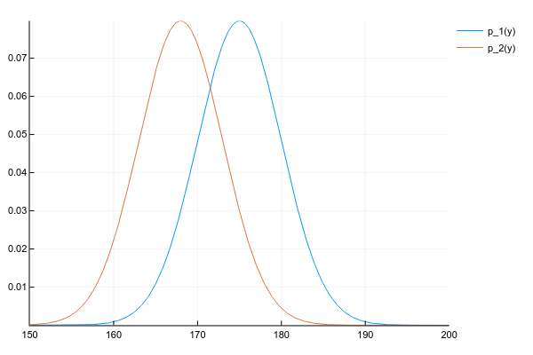
d1 = Normal(175, 5)
d2 = Normal(168, 5)
space = 150:0.1:200
y1 = [pdf(d1, y) for y inspace]
y2 = [pdf(d2, y) for y inspace]
plot(space, y1, label="p_1(y)")
plot!(space, y2, label="p_2(y)")
And we want to get their product:
p ( y ) = p 1 ( y ) p 2 ( y )
We know the probability density of both distributions at each point, therefore, honestly and in the general case, we need to multiply the density at each point. But, if we behaved well, thenp 1 ( y ) andp 2 ( y ) we have given the parameters, for example, for the normal distribution of 2 numbers - expectation and dispersion, and for their product will have to consider the probability at each point?
Fortunately, the product of many known distributions gives another known distribution with easily computable parameters. The key word here is conjugate prior .
No matter how we calculate, the product of two normal distributions gives one more normal distribution (though not normalized):
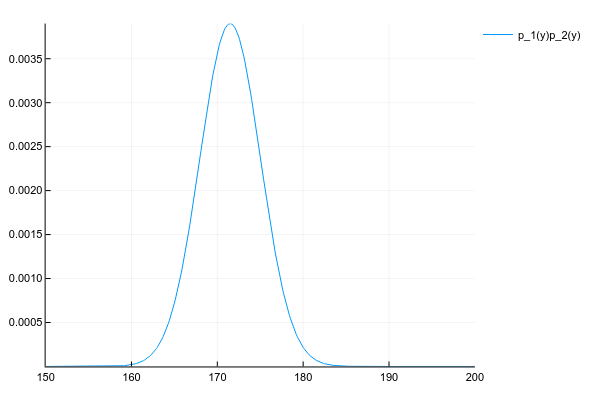
# честно перемножаем плотности вероятности в каждой точке# неэффективно, но работает для любых распределений
plot(space, y1 .* y2, label="p_1(y)p_2(y)")
Well, just for comparison, the distribution of the mixture of 3 normal distributions:

plot(space, [pdf(Normal(130, 5), x) for x in space] .+
                 [pdf(Normal(150, 20), x) for x in space] .+
                 [pdf(Normal(190, 3), x) for x in space])
Questions
Since this is a tutorial and someone will probably want to remember what was written here, here are a few questions for fixing the material.
Let human growth be a normally distributed random variable with parameters μ = 172 andσ 2 = 10 . What is the probability of meeting a person exactly 178cm tall?
Правильными ответами можно считать "0", "бесконечно мала" или "не определена". А всё потому что вероятность непрерывной переменной считается на некотором интервале. Для точки интервал — это её ширина, в зависимости от того, где вы учили математику, длину точки можно считать нулём, бесконечно малой или вообще не определённой.
Let be x - the number of children with the loan borrower (3 possible values),y - a sign of whether a person gave a loan (2 possible values). We use the Bayes formula to predict whether a particular customer with 1 child will give a loan. How many possible values can a priori and posterior distributions take, as well as likelihood and marginal likelihood?
Таблица совместного распредления двух переменных в данном случае небольшая и имеет вид:
| c=0 | c=1 | c=2 | |
|---|---|---|---|
| s=0 | p(s=0,c=0) | p(s=0,c=1) | p(s=0,c=2) |
| s=1 | p(s=1,c=0) | p(s=1,c=1) | p(s=1,c=2) |
где s — признак успешно отданного кредита.
Формула Байеса в данном случае имеет вид:
p(s|c)=p(c|s)p(s)p(c)
Если все значения известны, то:
- p(c) — это маргинальная вероятность увидеть человека с одним ребёнком, считается как сумма по колонке с=1 и является просто числом.
- p(s) — априорная/маргинальная вероятность того, что случайно взятый человек, про которого мы ничего не знаем, отдаст кредит. Может иметь 2 значения, соответствующих сумме по первой и по второй строке таблицы.
- p(c|s) — правдоподобие, условное распределение количества детей в зависимости от успешности кредита. Может показаться, что раз уж это распределение количества детей, то возможных значений должно быть 3, но это не так: мы уже точно знаем, что к нам пришёл человек с одним ребёнком, поэтому рассматриваем только одну колонку таблицы. А вот успешность кредита пока под вопросом, поэтому возможны 2 варианта — 2 строки таблицы.
- p(s|c) — апостериорное распределение, где мы знаем c, но рассматриваем 2 возможных варианта s.
Neural networks optimizing the distance between two distributions q ( x ) andp ( x ) , they often use cross entropy or Kullback-Leibler divergence distance as an optimization goal. The latter is defined as:
K L ( q | | p ) = ∫ q ( x ) log q ( x )p ( x ) dx
∫ q ( x ) ( . ) D x is the mat. waiting byq ( x ) , and why in the main part -log q ( x )p ( x ) - division is used, and not just the difference between the densities of two functionsq ( x ) - p ( x ) ?
logq(x)p(x)=logq(x)−logp(x)
Другими словами, это и есть разница между плотностями, но в логарифмическом пространстве, которе является вычислительно более стабильным.