Overview of the new UMAP dimension reduction algorithm. Is it really better and faster than t-SNE?
Hello, Habr! The task of reducing the dimension is one of the most important in the analysis of data and can arise in the following two cases. Firstly, for visualization purposes: before working with multidimensional data, it may be useful for a researcher to look at their structure, reducing the dimension and projecting them onto a two-dimensional or three-dimensional plane. Secondly, dimensionality reduction is useful for preprocessing features in machine learning models, since it is often inconvenient to train algorithms on a hundred features, among which there may be many noisy and / or linearly dependent ones, of course we would like to get rid of them. Finally, reducing the dimension of space greatly speeds up the training of models, and we all know that time is our most valuable resource.
UMAP (Uniform Manifold Approximation and Projection)- This is a new algorithm for reducing the dimension, the library with the implementation of which was released recently. The authors of the algorithm believe that UMAP can challenge modern models of dimensionality reduction, in particular, t-SNE, which is by far the most popular. According to the results of their research, UMAP has no restrictions on the dimension of the original feature space, which must be reduced, it is much faster and more computationally efficient than t-SNE, and also better copes with the task of transferring the global data structure to a new, reduced space.
In this article, we will try to understand what UMAP is, how to configure the algorithm, and finally, check whether it really has advantages over t-SNE.

Dimension reduction algorithms can be divided into 2 main groups: they try to preserve either the global data structure or local distances between points. The former include such algorithms as the Principal Component Method (PCA) and MDS (Multidimensional Scaling) , and the latter include t-SNE , ISOMAP , LargeVis and others. UMAP refers specifically to the latter and shows similar results to t-SNE.
Since a deep understanding of the principles of the algorithm requires strong mathematical training, knowledge of Riemannian geometry and topology, we describe only the general idea of the UMAP model, which can be divided into two main steps. At the first stage, we evaluate the space in which, by our assumption, the data is located. It can be set a priori (how simple ), or evaluate based on data. And at the second step we are trying to create a mapping from the space estimated at the first stage to a new, smaller dimension.
So, now let's try to apply UMAP to some data set and compare its visualization quality with t-SNE. Our choice fell on the Fashion MNIST dataset , which includes 70,000 black and white images of various clothes in 10 classes: t-shirts, trousers, sweaters, dresses, sneakers, etc. Each picture has a size of 28x28 pixels or 784 pixels in total. They will be features in our model.
So, let's try to use the UMAP library in Python in order to present our garments on a two-dimensional plane. We set the number of neighbors to 5, and leave the rest of the parameters by default. We will discuss them a bit later.
The transformation resulted in two vectors of the same length as the original dataset. We visualize these vectors and see how well the algorithm managed to preserve the data structure:
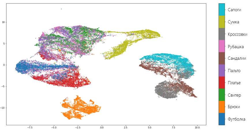
As you can see, the algorithm copes quite well and “did not lose” most of the valuable information that distinguishes one type of clothing from another. Also, the quality of the algorithm is also evidenced by the fact that UMAP separated shoes, torso and trousers from each other, realizing that these are completely different things. Of course, there are mistakes. For example, the model decided that a shirt and a sweater are one and the same.
Now let's see how t-SNE is managed with the same dataset. To do this, we will use Multicore TSNE - the fastest (even in single core mode) among all implementations of the algorithm:
Result:
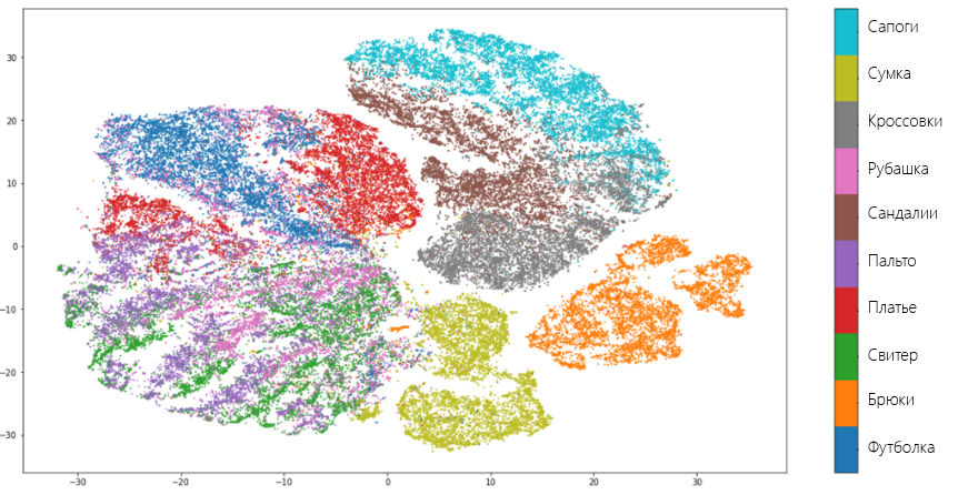
T-SNE shows similar results to UMAP and makes the same mistakes. However, unlike UMAP, t-SNE does not so clearly unite types of clothing in separate groups: trousers, things for the trunk and legs are close to each other. However, in general, we can say that both algorithms coped equally well with the task and the researcher is free to make one choice in favor of one or the other. It could have been if not for one “but”.
This “but” is the speed of learning. On a server with 4 Intel Xeon E5-2690v3 cores, 2.6 Hz and 16 GB of RAM on a data set of size 70000x784, UMAP learned in 4 minutes and 21 seconds , while t-SNE took almost 5 times as long : 20 minutes, 14 seconds. That is, UMAP is much more computationally efficient, which gives it a huge advantage over other algorithms, including t-SNE.
The number of neighbors is n_neighbors . By varying this parameter, you can choose what is more important to save in a new spatial representation of the data: global or local data structure. Small parameter values mean that, trying to estimate the space in which the data is distributed, the algorithm is limited to a small neighborhood around each point, that is, it tries to catch the local data structure (possibly to the detriment of the overall picture). On the other hand, large n_neighbors values force UMAP to account for points in a larger neighborhood, preserving the global data structure, but missing out on details.
Let's look at an example of our dataset how the n_neighbors parameter affects the quality and speed of training:
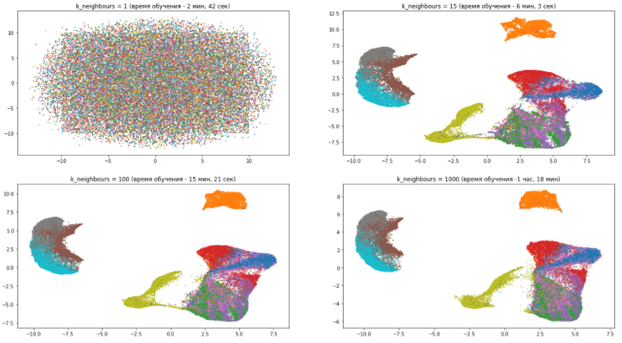
The following several conclusions can be drawn from this picture:
The minimum distance is min_dist . This parameter should be taken literally: it determines the minimum distance at which points in the new space can be. Low values should be used if you are interested in which clusters your data is divided into, and high values if it is more important for you to look at the data structure as a whole.
Let's go back to our dataset and evaluate the effect of the min_dist parameter . The n_neighbors value will be fixed and equal to 5:
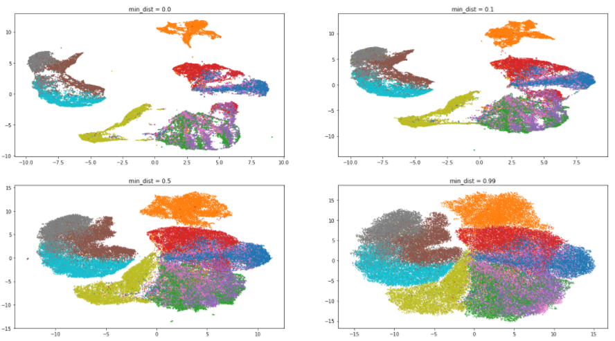
As expected, increasing the parameter value leads to a lesser degree of clustering, the data is collected in a heap and the differences between them are erased. Interestingly, with a minimum value of min_distthe algorithm tries to find the differences within the clusters and divide them into even smaller groups.
The distance metric is metric . The metric parameter determines how the distances in the source data space will be calculated. By default, UMAP supports all kinds of distances, from Minkowski to Hamming. The choice of metric depends on how we interpret this data and its type. For example, when working with textual information, it is preferable to use the cosine distance ( metric = 'cosine' ).
Let's continue playing with our dataset and try various metrics:
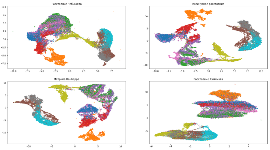
According to these pictures, you can make sure that the choice of a measure of distance greatly affects the final result, therefore, you need to approach its choice responsibly. If you are not sure which metric from the whole variety to choose, then the Euclidean distance is the safest option (it is by default in UMAP).
The dimension of the finite space is n_components . Everything is obvious here: the parameter determines the dimension of the resulting space. If you need to visualize the data, you should choose 2 or 3. If you use the converted vectors as features of machine learning models, you can do more.
UMAP was developed very recently and is constantly being improved, but now we can say that it is not inferior to other algorithms in the quality of work and may, finally, solve the main problem of modern models of decreasing dimensionality - slow learning.
Lastly, see how UMAP was able to visualize a Google News dataset of 3 million word vectors. The training time was 200 minutes, while t-SNE took several days:
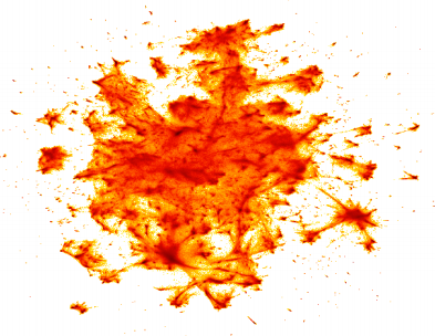
By the way, the picture was built using the datashader library for visualizing big data , which we will tell you in one of the following articles!
Among the algorithms for reducing the dimension is SVD, which we pay attention to in the context of building recommendations on our program "Big Data Specialist 8.0" , which starts on March 22.
UMAP (Uniform Manifold Approximation and Projection)- This is a new algorithm for reducing the dimension, the library with the implementation of which was released recently. The authors of the algorithm believe that UMAP can challenge modern models of dimensionality reduction, in particular, t-SNE, which is by far the most popular. According to the results of their research, UMAP has no restrictions on the dimension of the original feature space, which must be reduced, it is much faster and more computationally efficient than t-SNE, and also better copes with the task of transferring the global data structure to a new, reduced space.
In this article, we will try to understand what UMAP is, how to configure the algorithm, and finally, check whether it really has advantages over t-SNE.
Bit of theory
Dimension reduction algorithms can be divided into 2 main groups: they try to preserve either the global data structure or local distances between points. The former include such algorithms as the Principal Component Method (PCA) and MDS (Multidimensional Scaling) , and the latter include t-SNE , ISOMAP , LargeVis and others. UMAP refers specifically to the latter and shows similar results to t-SNE.
Since a deep understanding of the principles of the algorithm requires strong mathematical training, knowledge of Riemannian geometry and topology, we describe only the general idea of the UMAP model, which can be divided into two main steps. At the first stage, we evaluate the space in which, by our assumption, the data is located. It can be set a priori (how simple
), or evaluate based on data. And at the second step we are trying to create a mapping from the space estimated at the first stage to a new, smaller dimension.Application Results
So, now let's try to apply UMAP to some data set and compare its visualization quality with t-SNE. Our choice fell on the Fashion MNIST dataset , which includes 70,000 black and white images of various clothes in 10 classes: t-shirts, trousers, sweaters, dresses, sneakers, etc. Each picture has a size of 28x28 pixels or 784 pixels in total. They will be features in our model.
So, let's try to use the UMAP library in Python in order to present our garments on a two-dimensional plane. We set the number of neighbors to 5, and leave the rest of the parameters by default. We will discuss them a bit later.
import pandas as pd
import umap
fmnist = pd.read_csv('fashion-mnist.csv') # считываем данные
embedding = umap.UMAP(n_neighbors=5).fit_transform(fmnist.drop('label', axis=1)) # преобразовываем
The transformation resulted in two vectors of the same length as the original dataset. We visualize these vectors and see how well the algorithm managed to preserve the data structure:
As you can see, the algorithm copes quite well and “did not lose” most of the valuable information that distinguishes one type of clothing from another. Also, the quality of the algorithm is also evidenced by the fact that UMAP separated shoes, torso and trousers from each other, realizing that these are completely different things. Of course, there are mistakes. For example, the model decided that a shirt and a sweater are one and the same.
Now let's see how t-SNE is managed with the same dataset. To do this, we will use Multicore TSNE - the fastest (even in single core mode) among all implementations of the algorithm:
from MulticoreTSNE import MulticoreTSNE as TSNE
tsne = TSNE()
embedding_tsne = tsne.fit_transform(fmnist.drop('label', axis = 1))
Result:
T-SNE shows similar results to UMAP and makes the same mistakes. However, unlike UMAP, t-SNE does not so clearly unite types of clothing in separate groups: trousers, things for the trunk and legs are close to each other. However, in general, we can say that both algorithms coped equally well with the task and the researcher is free to make one choice in favor of one or the other. It could have been if not for one “but”.
This “but” is the speed of learning. On a server with 4 Intel Xeon E5-2690v3 cores, 2.6 Hz and 16 GB of RAM on a data set of size 70000x784, UMAP learned in 4 minutes and 21 seconds , while t-SNE took almost 5 times as long : 20 minutes, 14 seconds. That is, UMAP is much more computationally efficient, which gives it a huge advantage over other algorithms, including t-SNE.
Algorithm parameters
The number of neighbors is n_neighbors . By varying this parameter, you can choose what is more important to save in a new spatial representation of the data: global or local data structure. Small parameter values mean that, trying to estimate the space in which the data is distributed, the algorithm is limited to a small neighborhood around each point, that is, it tries to catch the local data structure (possibly to the detriment of the overall picture). On the other hand, large n_neighbors values force UMAP to account for points in a larger neighborhood, preserving the global data structure, but missing out on details.
Let's look at an example of our dataset how the n_neighbors parameter affects the quality and speed of training:
The following several conclusions can be drawn from this picture:
- With the number of neighbors equal to one, the algorithm works just awfully, because it focuses too much on the details and simply cannot catch the general data structure.
- With the increase in the number of neighbors, the model pays less attention to differences between different types of clothes, grouping similar ones and mixing them together. At the same time, completely different wardrobe items are getting farther apart. As already mentioned, the overall picture becomes clearer, and the details are blurred.
- The n_neighbors parameter significantly affects the training time. Therefore, you need to carefully approach its selection.
The minimum distance is min_dist . This parameter should be taken literally: it determines the minimum distance at which points in the new space can be. Low values should be used if you are interested in which clusters your data is divided into, and high values if it is more important for you to look at the data structure as a whole.
Let's go back to our dataset and evaluate the effect of the min_dist parameter . The n_neighbors value will be fixed and equal to 5:
As expected, increasing the parameter value leads to a lesser degree of clustering, the data is collected in a heap and the differences between them are erased. Interestingly, with a minimum value of min_distthe algorithm tries to find the differences within the clusters and divide them into even smaller groups.
The distance metric is metric . The metric parameter determines how the distances in the source data space will be calculated. By default, UMAP supports all kinds of distances, from Minkowski to Hamming. The choice of metric depends on how we interpret this data and its type. For example, when working with textual information, it is preferable to use the cosine distance ( metric = 'cosine' ).
Let's continue playing with our dataset and try various metrics:
According to these pictures, you can make sure that the choice of a measure of distance greatly affects the final result, therefore, you need to approach its choice responsibly. If you are not sure which metric from the whole variety to choose, then the Euclidean distance is the safest option (it is by default in UMAP).
The dimension of the finite space is n_components . Everything is obvious here: the parameter determines the dimension of the resulting space. If you need to visualize the data, you should choose 2 or 3. If you use the converted vectors as features of machine learning models, you can do more.
Conclusion
UMAP was developed very recently and is constantly being improved, but now we can say that it is not inferior to other algorithms in the quality of work and may, finally, solve the main problem of modern models of decreasing dimensionality - slow learning.
Lastly, see how UMAP was able to visualize a Google News dataset of 3 million word vectors. The training time was 200 minutes, while t-SNE took several days:
By the way, the picture was built using the datashader library for visualizing big data , which we will tell you in one of the following articles!
Among the algorithms for reducing the dimension is SVD, which we pay attention to in the context of building recommendations on our program "Big Data Specialist 8.0" , which starts on March 22.