Working with Anaconda using the example of cryptocurrency rate correlation search

The purpose of this article is to provide an easy introduction to data analysis using Anaconda. We will go through writing a simple Python script to extract, analyze and visualize data on various cryptocurrencies.

Step 1 - Setting up the work environment.

The only skills you'll need are a basic understanding of Python.

Step 1.1 - Installing Anaconda Anaconda

distribution can be downloaded from the official website .
Installation takes place in standard Step-by-Step mode.

Step 1.2 - Setting up the project work environment

After Anaconda is installed, you need to create and activate a new environment to organize our dependencies.

Why use environments? If you plan to develop several Python projects on your computer, it is useful to store dependencies (software libraries and packages) separately to avoid conflicts. Anaconda will create a special environment directory for the dependencies of each project so that everything is organized and divided.

You can do this either through the command line

conda create --name cryptocurrency-analysis python=3.6

source activate cryptocurrency-analysis

(Linux / macOS)

or

activate cryptocurrency-analysis

(Windows)

or through Anaconda Navigator



In this case, the environment is automatically activated.

Then you need to install the necessary dependencies NumPy , Pandas , nb_conda , Jupiter , Plotly , Quandl .

conda install numpy pandas nb_conda jupyter plotly quandl

либо через Anaconda Navigator, поочередно каждый пакет



Это может занять несколько минут.

Шаг 1.3 — Запуск Jupyter Notebook

Так же существует вариант через командную строку jupyter notebook и откройте браузер на http://localhost:8888/

и через Anaconda Navigator



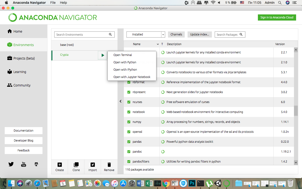
Шаг 1.4 — Импорт зависимостей

После того, как вы откроете пустой Jupyter Notebook, первое, что нужно сделать — это импорт необходимых зависимостей.

import os
import numpy as np
import pandas as pd
import pickle
import quandl
from datetime import datetime

Затем импорт и активация автономного режима Plotly.

import plotly.offline as py
import plotly.graph_objs as go
import plotly.figure_factory as ff
py.init_notebook_mode(connected=True)

Шаг 2 — Получение данных о ценах на биткоин

Now that everything is set up, we are ready to start extracting data for analysis. To begin with, we get price data using the free Quandl API.

Step 2.1 - Defining the Quandl Function We
begin by defining a function for loading and caching datasets from Quandl.

def get_quandl_data(quandl_id):
    '''Download and cache Quandl dataseries'''
    cache_path = '{}.pkl'.format(quandl_id).replace('/','-')
    try:
        f = open(cache_path, 'rb')
        df = pickle.load(f)   
        print('Loaded {} from cache'.format(quandl_id))
    except (OSError, IOError) as e:
        print('Downloading {} from Quandl'.format(quandl_id))
        df = quandl.get(quandl_id, returns="pandas")
        df.to_pickle(cache_path)
        print('Cached {} at {}'.format(quandl_id, cache_path))
    return df

We use pickle to serialize and save the downloaded data as a file, which allows our script not to reload the same data each time the script is run.

The function will return data as a pandas dataset.

Step 2.2 - Getting the Bitcoin exchange rate on the Kraken exchange We will

implement this as follows:

btc_usd_price_kraken = get_quandl_data('BCHARTS/KRAKENUSD')

To check the correctness of the script execution, we can look at the first 5 lines of the received answer using the head () method.

btc_usd_price_kraken.head()

Result:

Date	Open	High	Low	Close	Volume (BTC)	Volume (Currency)	Weighted Price
2014-01-07	874.67040	892.06753	810.00000	810.00000	15.622378	13151.472844	841.835522
2014-01-08	810.00000	899.84281	788.00000	824.98287	19.182756	16097.329584	839.156269
2014-01-09	825.56345	870.00000	807.42084	841.86934	8.158335	6784.249982	831.572913
2014-01-10	839.99000	857.34056	817.00000	857.33056	8.024510	6780.220188	844.938794
2014-01-11	858.20000	918.05471	857.16554	899.84105	18.748285	16698.566929	890.671709

And build a graph to visualize the resulting array

btc_trace = go.Scatter(x=btc_usd_price_kraken.index, y=btc_usd_price_kraken['Weighted Price'])
py.iplot([btc_trace])

Здесь мы используем Plotly для генерации наших визуализаций. Это менее традиционный выбор, чем некоторые из более известных библиотек, таких как Matplotlib, но я думаю, что Plotly — отличный выбор, поскольку он создает полностью интерактивные диаграммы с использованием D3.js.

Шаг 2.3 — Получение курса биткоина на нескольких биржах

Характер обмена заключается в том, что ценообразование определяется предложением и спросом, поэтому ни одна биржа не содержит «истинной цены» Биткойна. Чтобы решить эту проблему мы будем извлекать дополнительно данные из трех более крупных бирж для расчета совокупного индекса цены.

Мы будем загружать данные каждой биржи в словарь.

exchanges = ['COINBASE','BITSTAMP','ITBIT']
exchange_data = {}
exchange_data['KRAKEN'] = btc_usd_price_kraken
for exchange in exchanges:
    exchange_code = 'BCHARTS/{}USD'.format(exchange)
    btc_exchange_df = get_quandl_data(exchange_code)
    exchange_data[exchange] = btc_exchange_df

Шаг 2.4 — Объединение всех цен в единый набор данных

Определим простую функцию для объединения данных.

def merge_dfs_on_column(dataframes, labels, col):
    series_dict = {}
    for index in range(len(dataframes)):
        series_dict[labels[index]] = dataframes[index][col]
    return pd.DataFrame(series_dict)

Then combine all the data in the column "Weighted Price".

btc_usd_datasets = merge_dfs_on_column(list(exchange_data.values()), list(exchange_data.keys()), 'Weighted Price')

Now, let's look at the last five lines using the tail () method to make sure everything looks normal and the way we wanted.

btc_usd_datasets.tail()

Result:

Date	Bitstamp	COINBASE	ITBIT	Kraken	avg_btc_price_usd
2018-02-28	10624.382893	10643.053573	10621.099426	10615.587987	10626.030970
2018-03-01	10727.272600	10710.946064	10678.156872	10671.653953	10697.007372
2018-03-02	10980.298658	10982.181881	10973.434045	10977.067909	10978.245623
2018-03-03	11332.934468	11317.108262	11294.620763	11357.539095	11325.550647
2018-03-04	11260.751253	11250.771211	11285.690725	11244.836468	11260.512414

Step 2.5 - Compare Price Datasets.

The next logical step is to visualize the comparison of prices received. To do this, we will define an auxiliary function that will plot for each of the exchanges using Plotly.

def df_scatter(df, title, seperate_y_axis=False, y_axis_label='', scale='linear', initial_hide=False):
    label_arr = list(df)
    series_arr = list(map(lambda col: df[col], label_arr))
    layout = go.Layout(
        title=title,
        legend=dict(orientation="h"),
        xaxis=dict(type='date'),
        yaxis=dict(
            title=y_axis_label,
            showticklabels= not seperate_y_axis,
            type=scale
        )
    )
    y_axis_config = dict(
        overlaying='y',
        showticklabels=False,
        type=scale )
    visibility = 'visible'
    if initial_hide:
        visibility = 'legendonly'
    trace_arr = []
    for index, series in enumerate(series_arr):
        trace = go.Scatter(
            x=series.index, 
            y=series, 
            name=label_arr[index],
            visible=visibility
        )
        if seperate_y_axis:
            trace['yaxis'] = 'y{}'.format(index + 1)
            layout['yaxis{}'.format(index + 1)] = y_axis_config    
        trace_arr.append(trace)
    fig = go.Figure(data=trace_arr, layout=layout)
    py.iplot(fig)

And call her

df_scatter(btc_usd_datasets, 'Цена биткоина на биржах (USD) ')

Result:



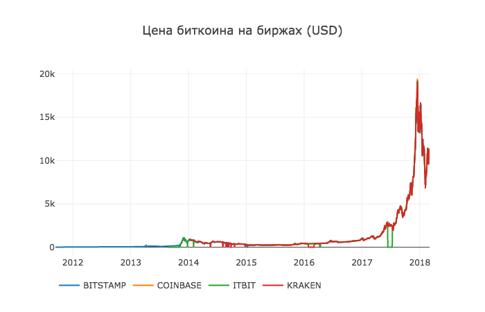
Now we delete all the zero values, since we know that the price has never been zero in the period we are considering.

btc_usd_datasets.replace(0, np.nan, inplace=True)

And re-create the schedule

df_scatter(btc_usd_datasets, 'Bitcoin Price (USD) By Exchange')

Result:



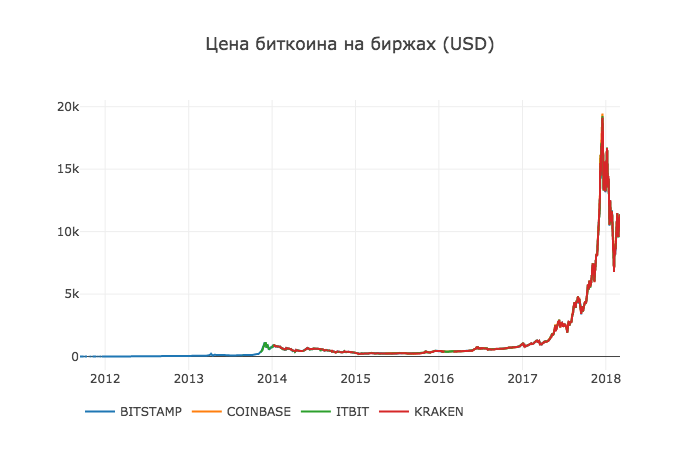
Step 2.6 - Calculating the average price

Now we can calculate a new column containing the average daily price of bitcoin on all exchanges.

btc_usd_datasets['avg_btc_price_usd'] = btc_usd_datasets.mean(axis=1)

This new column is our Bitcoin price index. We plot it to make sure it looks normal.

btc_trace = go.Scatter(x=btc_usd_datasets.index, y=btc_usd_datasets['avg_btc_price_usd'])
py.iplot([btc_trace])

Result:



We will use this data later to convert the exchange rates of other cryptocurrencies to USD.

Step 3 - Obtaining data on alternative cryptocurrencies

Now that we have an array of data with bitcoin prices, let's take some data on alternative cryptocurrencies.

Step 3.1 - Defining functions for working with the Poloniex API.

We will use the Poloniex API to get the data . We define two helper functions for loading and caching JSON data from this API.

First we define a function get_json_datathat will load and cache JSON data from the provided URL.

def get_json_data(json_url, cache_path):
    try:        
        f = open(cache_path, 'rb')
        df = pickle.load(f)   
        print('Loaded {} from cache'.format(json_url))
    except (OSError, IOError) as e:
        print('Downloading {}'.format(json_url))
        df = pd.read_json(json_url)
        df.to_pickle(cache_path)
        print('Cached response at {}'.format(json_url, cache_path))
    return df

Then we define a function to format the Poloniex API HTTP requests and call our new function get_json_datato save the received data.

base_polo_url = 'https://poloniex.com/public?command=returnChartData¤cyPair={}&start={}&end={}&period={}'
start_date = datetime.strptime('2015-01-01', '%Y-%m-%d') 
end_date = datetime.now() 
pediod = 86400 
def get_crypto_data(poloniex_pair):
    json_url = base_polo_url.format(poloniex_pair, start_date.timestamp(), end_date.timestamp(), pediod)
    data_df = get_json_data(json_url, poloniex_pair)
    data_df = data_df.set_index('date')
    return data_df

Эта функция на входе получает пару криптовалют например, «BTC_ETH» и вернет исторические данные по обменному курсу двух валют.

Шаг 3.2 — Загрузка данных из Poloniex

Некоторые из рассматриваемых альтернативных криптовалют нельзя купить на биржах напрямую за USD. По этой причине мы будем загружать обменный курс на биткоин для каждой из них, а затем будем использовать существующие данные о ценах биткоина для преобразования этого значения в USD.

Мы загрузим данные об обмене для девяти популярных криптовалют — Ethereum, Litecoin, Ripple, Ethereum Classic, Stellar, Dash, Siacoin, Monero, and NEM.

altcoins = ['ETH','LTC','XRP','ETC','STR','DASH','SC','XMR','XEM']
altcoin_data = {}
for altcoin in altcoins:
    coinpair = 'BTC_{}'.format(altcoin)
    crypto_price_df = get_crypto_data(coinpair)
    altcoin_data[altcoin] = crypto_price_df

Now we have 9 data sets, each of which contains historical average daily exchange ratios of bitcoins to alternative cryptocurrencies.

We can look at the last few rows of the Ethereum pricing table to make sure it looks normal.

altcoin_data['ETH'].tail()

date	close	high	low	open	quoteVolume	volume	weightedAverage
2018-03-01	0.079735	0.082911	0.079232	0.082729	17981.733693	1454.206133	0.080871
2018-03-02	0.077572	0.079719	0.077014	0.079719	18482.985554	1448.732706	0.078382
2018-03-03	0.074500	0.077623	0.074356	0.077562	15058.825646	1139.640375	0.075679
2018-03-04	0.075111	0.077630	0.074389	0.074500	12258.662182	933.480951	0.076149
2018-03-05	0.075373	0.075700	0.074723	0.075277	10993.285936	826.576693	0.075189

Step 3.3 - Convert prices to USD.

Since now we have a bitcoin exchange rate for each cryptocurrency and we have a historical bitcoin price index in USD, we can directly calculate the price in USD for each alternative cryptocurrency.

for altcoin in altcoin_data.keys():
    altcoin_data[altcoin]['price_usd'] =  altcoin_data[altcoin]['weightedAverage'] * btc_usd_datasets['avg_btc_price_usd']

With this, we created a new column in each data set of alternative cryptocurrencies with prices in USD.

Then we can reuse our function merge_dfs_on_columnto create a combined set of price data in USD for each cryptocurrency.

combined_df = merge_dfs_on_column(list(altcoin_data.values()), list(altcoin_data.keys()), 'price_usd')

Now add the bitcoin prices to the dataset as the final column.

combined_df['BTC'] = btc_usd_datasets['avg_btc_price_usd']

As a result, we have a data set containing daily USD prices for the ten cryptocurrencies we are considering.

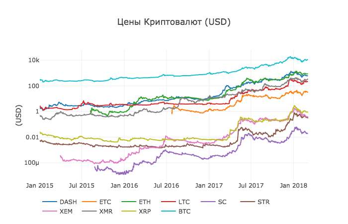
We use our function df_scatterto display all cryptocurrency prices on a chart.

df_scatter(combined_df, 'Цены Криптовалют (USD)', seperate_y_axis=False, y_axis_label='(USD)', scale='log')

This graph gives a pretty solid “overall picture” of how the exchange rates of each currency have changed over the past few years.



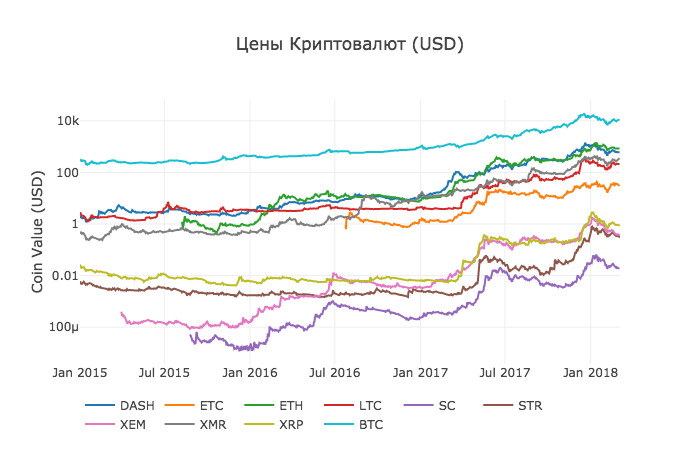
In this example, we use the Y-axis logarithmic scale to compare all currencies in the same section. You can try different parameter values ​​(for example, scale = 'linear') to get different points of view on the data.

Step 3.4 - Calculation of the cryptocurrency correlation.

You may notice that cryptocurrency exchange rates, despite their completely different values ​​and volatility, seem slightly correlated. And as you can see from the surge in April 2017, even small fluctuations seem to occur synchronously throughout the market.

We can test our correlation hypothesis using the Pandas methodcorr (), which calculates the Pearson correlation coefficient for each column in the data set with respect to each other. In the calculation, we also use a method pct_change ()that converts each cell in the data set from the absolute value of the price to a percentage change.

First we calculate the correlations for 2016.

combined_df_2016 = combined_df[combined_df.index.year == 2016]
combined_df_2016.pct_change().corr(method='pearson')

Result:

	Dash	Ect	Et	LTC	SC	STR	Xem	XMR	Xrp	BTC
Dash	1.000000	0.003992	0.122695	-0.012194	0.026602	0.058083	0.014571	0.121537	0.088657	-0.014040
Ect	0.003992	1.000000	-0.181991	-0.131079	-0.008066	-0.102654	-0.080938	-0.105898	-0.054095	-0.170538
Et	0.122695	-0.181991	1.000000	-0.064652	0.169642	0.035093	0.043205	0.087216	0.085630	-0.006502
LTC	-0.012194	-0.131079	-0.064652	1.000000	0.012253	0.113523	0.160667	0.129475	0.053712	0.750174
SC	0.026602	-0.008066	0.169642	0.012253	1.000000	0.143252	0.106153	0.047910	0.021098	0.035116
STR	0.058083	-0.102654	0.035093	0.113523	0.143252	1.000000	0.225132	0.027998	0.320116	0.079075
Xem	0.014571	-0.080938	0.043205	0.160667	0.106153	0.225132	1.000000	0.016438	0.101326	0.227674
XMR	0.121537	-0.105898	0.087216	0.129475	0.047910	0.027998	0.016438	1.000000	0.027649	0.127520
Xrp	0.088657	-0.054095	0.085630	0.053712	0.021098	0.320116	0.101326	0.027649	1.000000	0.044161
BTC	-0.014040	-0.170538	-0.006502	0.750174	0.035116	0.079075	0.227674	0.127520	0.044161	1.000000

Coefficients close to 1 or -1 mean that the data is strongly correlated or inversely correlated, respectively, and coefficients close to zero mean that the values ​​tend to fluctuate independently of each other.

To visualize these results, we will create another helper function.

def correlation_heatmap(df, title, absolute_bounds=True):
    heatmap = go.Heatmap(
        z=df.corr(method='pearson').as_matrix(),
        x=df.columns,
        y=df.columns,
        colorbar=dict(title='Pearson Coefficient'),
    )
    layout = go.Layout(title=title)
    if absolute_bounds:
        heatmap['zmax'] = 1.0
        heatmap['zmin'] = -1.0
    fig = go.Figure(data=[heatmap], layout=layout)
    py.iplot(fig)

correlation_heatmap(combined_df_2016.pct_change(), "Корреляция криптовалют (2016)")

Here, the dark red values ​​represent strong correlations, and the blue values ​​represent strong inverse correlations. All other colors represent varying degrees of faint / nonexistent correlations.

What does this chart tell us? In fact, this shows that there was very little statistically significant relationship between how the prices of different cryptocurrencies fluctuated during 2016.

Now, to test our hypothesis that cryptocurrencies have become more correlated in recent months, let us repeat the same tests using data from 2017 and 2018.

combined_df_2017 = combined_df[combined_df.index.year == 2017]
combined_df_2017.pct_change().corr(method='pearson')

Result:

	Dash	Ect	Et	LTC	SC	STR	Xem	XMR	Xrp	BTC
Dash	1.000000	0.387555	0.506911	0.340153	0.291424	0.183038	0.325968	0.498418	0.091146	0.307095
Ect	0.387555	1.000000	0.601437	0.482062	0.298406	0.210387	0.321852	0.447398	0.114780	0.416562
Et	0.506911	0.601437	1.000000	0.437609	0.373078	0.259399	0.399200	0.554632	0.212350	0.410771
LTC	0.340153	0.482062	0.437609	1.000000	0.339144	0.307589	0.379088	0.437204	0.323905	0.420645
SC	0.291424	0.298406	0.373078	0.339144	1.000000	0.402966	0.331350	0.378644	0.243872	0.325318
STR	0.183038	0.210387	0.259399	0.307589	0.402966	1.000000	0.339502	0.327488	0.509828	0.230957
XEM	0.325968	0.321852	0.399200	0.379088	0.331350	0.339502	1.000000	0.336076	0.268168	0.329431
XMR	0.498418	0.447398	0.554632	0.437204	0.378644	0.327488	0.336076	1.000000	0.226636	0.409183
XRP	0.091146	0.114780	0.212350	0.323905	0.243872	0.509828	0.268168	0.226636	1.000000	0.131469
BTC	0.307095	0.416562	0.410771	0.420645	0.325318	0.230957	0.329431	0.409183	0.131469	1.000000

correlation_heatmap(combined_df_2017.pct_change(), "Корреляция криптовалют (2017)")

combined_df_2018 = combined_df[combined_df.index.year == 2018]
combined_df_2018.pct_change().corr(method='pearson')

	DASH	ETC	ETH	LTC	SC	STR	XEM	XMR	XRP	BTC
DASH	1.000000	0.775561	0.856549	0.847947	0.733168	0.717240	0.769135	0.913044	0.779651	0.901523
ETC	0.775561	1.000000	0.808820	0.667434	0.530840	0.551207	0.641747	0.696060	0.637674	0.694228
ETH	0.856549	0.808820	1.000000	0.700708	0.624853	0.630380	0.752303	0.816879	0.652138	0.787141
LTC	0.847947	0.667434	0.700708	1.000000	0.683706	0.596614	0.593616	0.765904	0.644155	0.831780
SC	0.733168	0.530840	0.624853	0.683706	1.000000	0.615265	0.695136	0.626091	0.719462	0.723976
STR	0.717240	0.551207	0.630380	0.596614	0.615265	1.000000	0.790420	0.642810	0.854057	0.669746
XEM	0.769135	0.641747	0.752303	0.593616	0.695136	0.790420	1.000000	0.744325	0.829737	0.734044
XMR	0.913044	0.696060	0.816879	0.765904	0.626091	0.642810	0.744325	1.000000	0.668016	0.888284
XRP	0.779651	0.637674	0.652138	0.644155	0.719462	0.854057	0.829737	0.668016	1.000000	0.712146
BTC	0.901523	0.694228	0.787141	0.831780	0.723976	0.669746	0.734044	0.888284	0.712146	1.000000

correlation_heatmap(combined_df_2018.pct_change(), "Корреляция криптовалют (2018)")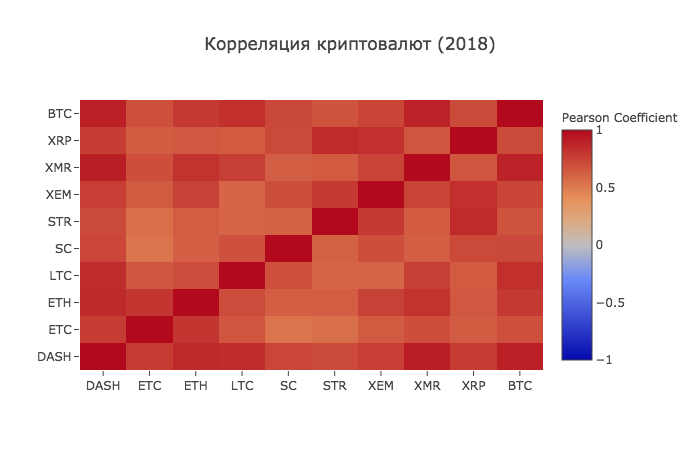

And now we see what we assumed - almost all cryptocurrencies have become more interconnected with each other in all directions.

On this, we assume that the introduction to working with data in Anaconda has been successfully completed.