February 19, 2018 at 14:18
Visualization of data for moviegoers: we scrap the recommendations of films and make an interactive graph
- Tutorial
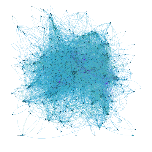
Once I came across an interactive lastfm map and decided to definitely make a similar project for films. Under the cut, the story is about how to collect data, build a graph and create your own interactive demo using data from film search and imdb as an example. We will look at the Scrapy scrapbooking framework, go over the methods of visualizing large graphs and deal with tools for interactively displaying large graphs in the browser.
1. Data Collection: Scrapy
As a data source, I chose cinema search. However, then it turned out that this is very small and I scraped up IMDb. To make a graph, for each movie you need to know the list of recommended films. If you search, you can find enough movie search parsers and all kinds of unofficial api, but nowhere is there any way to get recommendations. IMDb is openly sharing its dataset, but there are no recommendations. Therefore, there is only one choice: write your spider.
There are already several articles on scraping on the hub, so I'll skip the overview of possible approaches. In a nutshell: if you are writing in python and don't want to write your framework, use Scrapy . Almost everything that you may need is already provided in it.
Scrapy is really a very powerful and at the same time very simple tool. The entry threshold is quite low, but at the same time, Scrapy easily scales to projects of any size and complexity. It really contains everything you need. From tools for directly parsing and HTTP requests, processing and saving received elements, to managing the project, including ways to bypass the block, pause and resume scraping, etc.
Creating a project begins with a team scrapy startproject mycoolproject, after which you get a ready-made structure with templates of the necessary elements and files of a minimal working configuration. To make a working project out of this, it’s enough to describe how to pars the page — that is, create a spider and put it in a folder spidersinside the project, and describe what kind of information you want to extract — that is, inherit your class from the class scrapy.itemin the script items.py. Thus, you can make a fully working project in less than an hour. There are built-in tools for saving the results: for example, writing to csv or json, but it is better to use an external database if the project is not for five minutes. The behavior associated with the processing of results, including saving, is specified in pipelines.py. The last important file remains -settings.pythe purpose of which is clear from the name. Here you can specify the configuration of the project associated with, for example, the use of a proxy, timing between requests and much more.
And so, in steps:
- We look in the articles once , twice and in the documentation how to create a project for Scrapy. By analogy, we create our own class for items.
import scrapy
class MovieItem(scrapy.Item):
    '''Movie scraped info'''
    movie_id = scrapy.Field()
    name = scrapy.Field()
    like = scrapy.Field()
    genre = scrapy.Field()
    date = scrapy.Field()
    country = scrapy.Field()
director = scrapy.Field()- We look for the elements we need on the page and get them xpath. This can be done, for example, through chrome: right-click on an element, select inspect element, in the code, right-click again, and look for copy -> xpath. For debugging, you can run scrapy-shell and pass it url page
scrapy-shell https://www.kinopoisk.ru/film/518214/. You will instantiate a response object from which you can obtain the necessary elements.
$scrapy-shell https://www.kinopoisk.ru/film/sakhar-i-korica-1915-201125/
$response.xpath('//span[@itemprop="director"]/a/span/text()').extract_first()
'Эрнст Любич'- We customize the processing of the received objects. I chose to save the entry to the sqlite database, because it is very simple.
- We check that everything works by setting a parameter at startup
CLOSESPIDER_PAGECOUNT=5to limit the number of requests. - To battle! Create a directory to save intermediate results, for example
crawls1. We start the spider with the parameterscrapy crawl myspider -s JOBDIR=crawls1: now, if something goes wrong, we can restart the spider from the same place where it ended. The relevant section in the documentation .
1.1 Bypassing the limit on the number of requests.
Kinopoisk banned me at the stage of debugging a spider, when I sent a pack of 5 requests every 5 minutes with a timeout of 1 second. There are many options to get around the limitations. For scrapie, ready-made examples of using a torus, randomly sorting proxies from a list, or connecting to paid rotating proxy services are easy to google. Since we have a “weekend project”, I chose a rotating proxy - the fastest option to implement, though I have to connect to a paid service. How it works: you connect to a specific ip: port of your proxy provider, and at the output you get a new ip for each request. On the scrapy side, you need to add one line in the settings.py file of your project and pass a parameter for the ip: port pair in each request.
We look for the appropriate section in settings.py and add the line there:
DOWNLOADER_MIDDLEWARES = {
    'scrapy.downloadermiddlewares.httpproxy.HttpProxyMiddleware':543
}
Then in each request of your spider:
scrapy.Request(url=url, callback=self.parse,
                meta={'proxy':'http://YOU_RPROXY_IP:PORT'})
The author of the project that inspired me started with Nightwish and then went around lastfm's recommendations as wide as a tree - so he got a connected graph. My approach was similar. From cinema search you can get movies by id, which seems to simply correspond to the serial number of the movie on the site. If you just take all the ids, it will not work out very well, because most films do not have recommendations and will be single points that will turn into noise on the map. IDs of fresh films are of the order of 500,000 - this is quite a lot for visual rendering, so let's start with the list of top 250 films and iteratively go around the recommendation lists of each film.
I expected to get about 100,000 films, but by the end of the scraping night it turned out that the spider had stopped at ~ 12,600. The recommendations in the movie search end there. As mentioned at the beginning, I got on IMDb for new data. Scraping IMDb is even easier. A couple of hours to rewrite the finished project and a new spider is ready to start. After two or three days of crawling (8 requests per second, so as not to become impudent), the spider stopped, collecting 173+ thousand films. The full code of the spiders can be viewed on the github: film search and IMDb .
2. Visualization
On the one hand, graph visualization tools are a whole zoo. On the other hand, when it comes to very large graphs, this zoo suddenly runs up somewhere. I chose two tools for myself for such cases: these are sfdp from graphviz and gephi . SFDP is a CLI utility with a wide range of parameters, it is able to draw graphs per million nodes, but in our case it is not the most convenient tool, because we need to control the styling process. For cases like ours, Gephi is great - it's an application with a graphical interface and a universal set of styling, almost for every taste.
Exporting data for a graph is done with a simple python script. I usually use the dot format because it is very simple, called "human readable". Initially, the format is intended for use in graphviz, but now it is supported by many other graph applications.
Description of the format
At the beginning we write the title digraph kinopoisk {\nand do not forget to write a closing bracket at the end of the file }. In each line we describe the edges of the graph node1 -> node2;and close the list. Description of the format here: official docks and simple examples on Wikipedia .
digraph sample {
1 -> 2;
1 -> 3;
5 -> 4 [weight="5"];
4 [shape="circle"];
}digraph- means that we declare a directed graph. If you need not directed, then we write simply graph. sampleIs the name of our graph (optional). In each line, edges or vertices are declared. If the edges are not directed, then ->we write instead --. In square brackets, you can declare edge or vertex parameters. In this example, we set the edge between nodes 5 and 4 to be equal to five, and to the vertex 4 the shape of a circle. The names of the vertices do not have to be denoted by numbers; these can be strings. See the documentation for more examples and parameters. In our case, the capabilities described above are quite enough.
2.1 Comparison of styling
For large graphs, gephi has two reasonable options: OpenOrd and ForceAtlas 2. OpenOrd is a very fast approximate algorithm, but has few configurable parameters. ForceAtlas is similar to other classical force-directed algorithms, it gives more accurate results, it is very flexible in tuning, but you have to pay time for this. Below are examples of the operation of both algorithms on a graph representing a grid.


Model graph grid. Left OpenOrd, right ForceAtlas.
You might think that OpenOrd should not be used at all if you have time to wait for a more accurate result. In fact, graphs are not uncommon when ForceAtlas collects all nodes into one tight lump, and OpenOrd shows at least some kind of structure.
To speed up the process, I used OpenOrd as an initial approximation and then smeared the graph with ForceAtlas. In order for the image to be at least something clear, you need to eliminate the overlapping nodes on each other. For this, it is convenient to use the Yifan Hu stacking - to smudge the cluster a bit, and noverlap to completely eliminate the overlap. It took a night to eliminate the overlap in the cinema search column, and they could not cope with imdb for the whole weekend.


3. Export Results: Interactive Map
Gephi can export images to svg, png and many other formats. But big data comes with big difficulties. Beautiful pictures alone are not enough. We want to see the names of the films and how they are related. If we draw node labels, then with so many of them we get a completely unreadable cloud of letters. There are options to use SVG and scale it until something becomes visible, or draw only the most important labels. But there is a better option, which I decided to focus on. We make an interactive map.
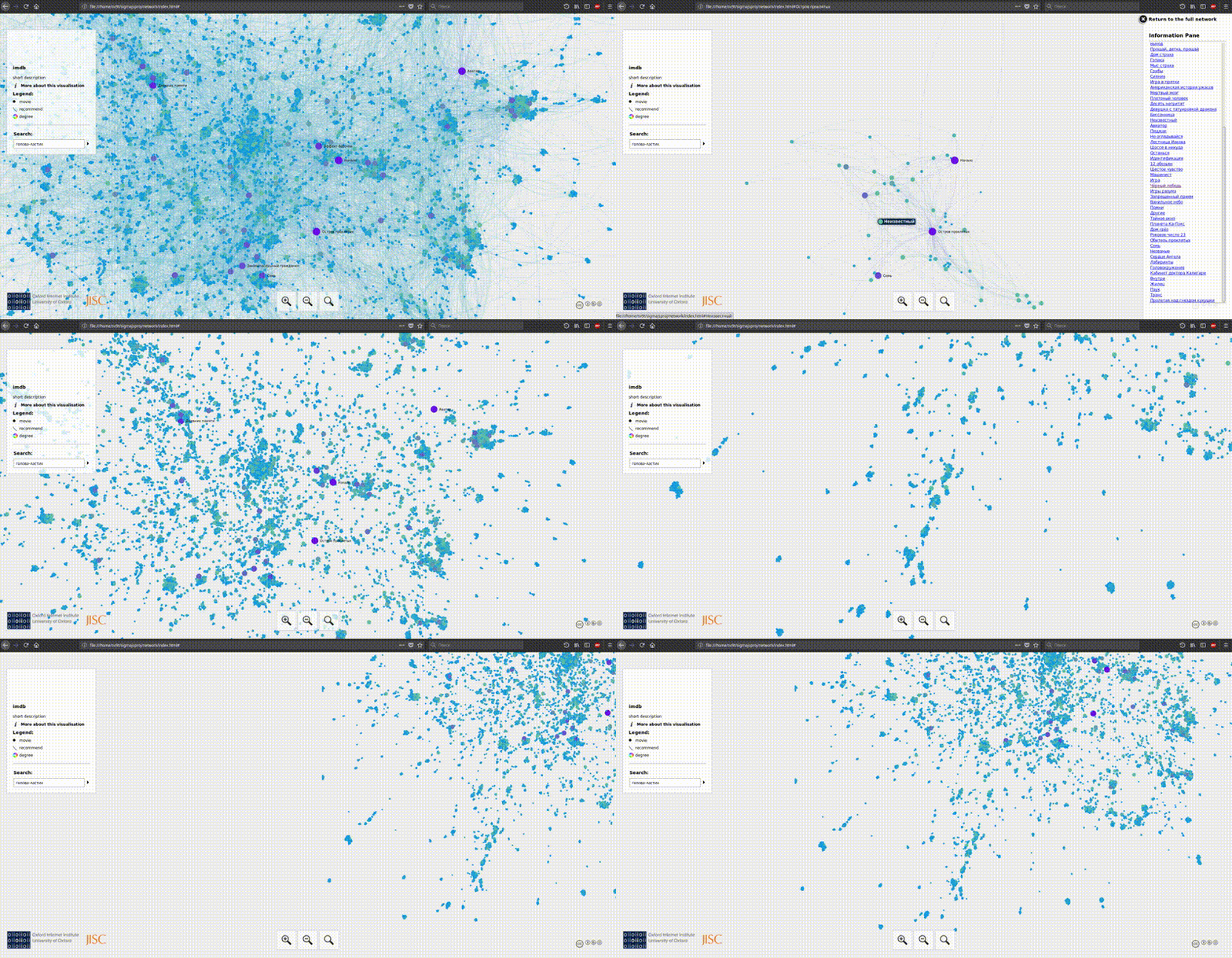
Tools Overview:
sigma.js
The first option, one of the simplest and at the same time the most intuitive, is a plugin for gephi with export to a sigma.js template. On the gif above it is just that. Install the plugin through the gephi menu, after which we have a new export menu item in the file tab. We fill out the form, export and get a ready-made working visualization. Simple and powerful. The result can be seen here . Disadvantage: on large graphs, the browser barely copes.
gefx-js
The next option is even simpler than the previous one and is generally very similar. gefx-js - you just need to export your project from gephi to gexf format and put it in the template folder. Done. The disadvantage is exactly the same as in the previous case. Moreover, if using sigmajs I could look at the imdb graph at least locally, then with gefx-js it just did not boot.
openseadragon
For cases when you need to show a very large picture, there is seadragon . The principle is exactly the same as when rendering geographical maps: when scaling, new tiles are loaded that correspond to the current increase and viewing area. That is exactly what the author of the project that inspired me did. One drawback: minimum interactivity. It is impossible to select nodes, it is difficult to see where the ribs go. It is impossible to “peek behind” the overlapping nodes and edges.
shinglejs
And what if you make something like a mixture of the previous options, so that when scaling the graph is loaded with tiles, but not with pictures, but as in the first case, with the interactivity of nodes and edges? The ready-made solution was found literally by a miracle, these are shinglejs .
Pros: you can render very (very, very) large graphs in the browser, while maintaining interactivity.
Cons: Not as beautiful as sigmages; preparing data is not trivial.

Not so beautiful, but very smart
To visualize the imdb graph, I chose the last option. In general, there was no choice. You can see the result here , and then a little about how to prepare data for such a visualization.
Exporting data to shinglejs:
As I said, exporting data in the latter case is not very simple, so I will give an example of how to unload a graph from gephi for shinglejs.
- Exporting a graph from gephi in gdf format - this is probably the only simple way to get the coordinates of nodes in the form of a table. The file structure is this: first comes a table with a description of the nodes, then a table with a description of the edges.
- We read the file and get the description of the vertices and edges from it. I did this with pandas, then chopped the data frame into two: edges and nodes. About working with pandas .
- We change the names of the columns in accordance with the shinglejs docks and export to json. Shinglejs does not support direct export of colors, but for each node you can specify "communities" and color them already. That’s why we upload movie ratings as community tags.
- In the sources of the main page, do not forget to specify a list of colors for the communities. For dyeing unit from the color list is taken from the item number which is calculated as follows:
id сообщества % количество цветов. - We glue the files into one. I did this through bash:
cat start imdbnodes.json middle imdbedges.json end > imdbdata.jsonhaving previously created the files with thestart, middle, stopcontents of "{"nodes":", ", "relations":" and "}" respectively. - Further according to the instructions from the office. site
- Do not forget to create a bitmap and put it in the graph data folder, otherwise at a great distance you will see only a few nodes or nothing at all. The author of the project does not seem to have indicated this detail, but by default the example will try to load the files
image_2400.jpgandimage_1200.jpg, rather than npm, as it might seem after building the default project.
4. Interesting observations
The lastfm column has a clear clustering associated with the countries of origin of musical groups, for example, Japanese pop and rock, Greek metal, etc. Exactly the same thing happens with films. Korean cinema, Turkish, Japanese and Brazilian are very clearly separated. In imdb, far from the main mass, a large cluster of cartoons stands out. On both graphs, a cluster of comic book superhero films is very tightly packed. It seems to be obvious, but nonetheless unexpected, that bad films gather in one big cloud. There are separate clusters of music videos, children's youtube blogs and fan films about the Harry Potter universe.
5. What else can be done with this data
I am sure that readers will be able to come up with and do many more interesting projects on the received data. I immediately get the following ideas:
- Cluster and compile collections. DBSCAN worked fine for me almost from the first run. (An example will follow)
- Make your own recommendation systems
- Collect interesting statistics about movies in general
- Of course, expand your film library.
5.1 DBSCAN
There are many special methods for clustering graphs, and all of them are worthy of separate articles. As an experiment, I used a method not intended for graphs. The reasoning was as follows: once the graph has visually decomposed into clouds of similar films, the areas where the films are especially close to each other can be found using DBSCAN . Let's see what this method does without going into deep details. The name DBSCAN stands for density-based scan, that is, using this method, we merge the points that are located fairly closely together. This is formalized through two main hyperparameters - this is the radius in which we look for neighbors for each point and the minimum number of neighbors.
1. Get the coordinates.
To do this, we export our graph from gephi in gdf format. We read the file as csv using pandas:
data = pd.read_csv('./kinopoisk.gdf')
# gdf содержит как-бы два файла в одном
# сначала описание вершин, а потом описание рёбер
# pandas читает это как целый файл, а недостающие поля в конце
# заполняет как nan поэтому можно достать информацию о вершинах например вот так
data_nodes = data[data['y DOUBLE'].apply(lambda x: not np.isnan(x))]
Let's draw and see what it looks like.
plt.figure(figsize=(7, 7))
plt.scatter(data['x DOUBLE'].values, data['y DOUBLE'].values, marker='.', alpha=0.3);
Well, DBSCAN should handle that.
2. Cluster.
We select the parameters and look at the distribution of cluster sizes. No serious work was planned, so I evaluated the quality "by eye".
from sklearn.cluster import DBSCAN
coords = data_nodes[['x DOUBLE', 'y DOUBLE']].values
dbscan = DBSCAN(eps=70, min_samples=5, leaf_size=30, n_jobs=-1)
labels = dbscan.fit_predict(coords)
plt.hist(labels, bins=50);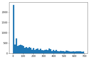
Cluster size distribution
Let's colorize our points in the colors of the clusters and see how the result looks like the truth.
plt.figure(figsize=(8, 8))
for l in set(labels):
    coordsm = coords[labels == l]
    plt.scatter(coordsm[:,0], coordsm[:,1], marker='.', alpha=0.3);
It looks like what we wanted to get.
Let's try to get a cluster of a movie in the form of a list. I did not take care to make a convenient way to get the list, so this time without code. Below is a list of films that fell into one cluster with "real ghouls." In my opinion, not bad.
| movie_id | name | date | genre | country | director |
|---|---|---|---|---|---|
| 271695 | Third planet from the sun | 1996-01-09 | fantasy | USA | Terry Hughes |
| 663135 | Neighbors | 2012-09-26 | comedy | USA | Chris Koch |
| 277375 | Aliens | 1997-11-07 | cartoon | France | Jim Gomez |
| 81845 | Sweeney Todd, the demon barber of Fleet Street | 2007-12-03 | musical | USA | Tim Burton |
| 445196 | Hands and feet for love | 2010-10-29 | thriller | Great Britain | John Landis |
| 271878 | Red hotel | 2007-12-05 | comedy | France | Gerard Kravchik |
| 3609 | Plunkett and MacLane | 1999-01-22 | action movie | Great Britain | Jake scott |
| 183497 | Bourke and Hare | 1972-02-03 | horrors | Great Britain | Vernon Sewell |
| 3482 | Doctor and the Devils | 1985-10-04 | horrors | Great Britain | Freddy francis |
| 2528 | Addams Family Values | 1993-11-19 | fantasy | USA | Barry Sonnenfeld |
| 503578 | Lullaby | 2010-02-12 | fantasy | Poland | Juliusz Makhulsky |
| 87404 | Red tavern | 1951-10-19 | comedy | France | Claude Otan Lara |
| 5293 | Addams Family | 1991-11-22 | fantasy | USA | Barry Sonnenfeld |
| 18089 | Body Thieves | 1945-02-16 | horrors | USA | Robert Wise |
| 271846 | Seller of the dead | 2008-10-10 | horrors | USA | Glenn McQueid |
| 272111 | Freshly buried | 2007-09-09 | drama | Canada | Chaz Thorne |
| 34186 | Elvira: Queen of Darkness | 1988-09-30 | comedy | USA | James Signorelli |
| 818981 | Real ghouls | 2014-01-19 | comedy | New Zealand | Jamain Clement |
| 8421 | Edward Scissorhands | 1990-12-06 | fantasy | USA | Tim Burton |
| 5622 | Sleepy Hollow | 1999-11-17 | horrors | USA | Tim Burton |
| 2389 | Beatlejus | 1988-03-29 | fantasy | USA | Tim Burton |
This approach seems interesting to me because we get a list of similar films that are not necessarily related to direct recommendations, and are not even reachable in a small number of steps when traversing the graph. That is, so you can find a movie that gets caught just by clicking on similar films directly on the site.
PS
Thanks to all friends who were ready to answer my questions, to all moviegoers - new discoveries, and high-quality data to datacents!