Verhulst on bitcoin
- Tutorial
Bitcoin and other cryptocurrencies have captured the attention of a huge number of people. Why not take this chance to popularize mathematics and, in particular, Mathcad? In this article, we will consider several simple well-known models based on differential equations, namely, a family of logistic models (unlimited growth, with competition for a resource, with a fishery and a delay). For the first time, the Belgian mathematician Ferhulst proposed the systemic factor limiting the growth of the biological population, therefore the corresponding model (it will be considered the second in a row) rightly bears his name.
Since everything that has been happening lately with bitcoin looks like a pyramid, the models will be appropriate, especially since many colleagues, for example, M. Balandin and V. , devoted their articles to the mathematical apparatus, thanks to MMM . Points . We will pay the main attention, as before, to the methods of calculations in Mathcad, especially in its free version of Mathcad Express , without insisting on the accuracy of the forecast, what the bitcoin exchange rate will be in the near future, and when exactly it will crash.
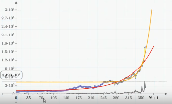
First of all, it is worth noting that so far, over the past few months, the graph of the Bitcoin exchange rate has strongly resembled exponential growth (see the graph above). Those. it begs the use of an equation of the type y '(t) = S * y (t), the solution of which is an exponential function. To be able to compare experimental data and simulation results in Mathcad, you must first import the source data into a Mathcad document. To how this is done (by the way, import also works in the free version of Mathcad Express) I dedicated a screencast in which I also showed how data can be interpolated and extrapolated using an exponential function. The result of interpolation-extrapolation is shown in the upper graph of the red (according to the data for the last year) and orange (4 months) curves.
In this article, we will calculate several simple well-known models based on ordinary differential equations . They were originally proposed as models of the growth of biological populations (see in more detail, for example, here), and subsequently began to be used to model epidemics, as well as economic phenomena similar to this one. The first model is y '(t) = S * y (t), where y (t) - we consider the bitcoin exchange rate at time t. This world famous model was proposed by Malthus in 1798 in his classic work On the Law of Population Growth. If we draw an analogy with the dynamics of the population, or rather, with the spread of the epidemic, then y (t) would be more adequate to consider the total capitalization of Bitcoin, i.e. value of the current rate multiplied by the number of bitcoins. But since the number of bitcoins has changed little over the year (and it has increased due to mining), for simplicity and clarity, y (t) can be considered the current rate.
We turn now to the next model - the Verhulst equation y '= S * y - k * y 2, in which the last term describes the attenuation of the epidemic due to resource limitations. Accordingly, let's look at this example how in mathcad prime and mathcad express it is possible to solve ordinary differential equations (hereinafter ODE). In the fully functional version of mathcad prime, a “solution block” is used for this, in which the initial condition is written, the differential equation itself (it is highlighted in yellow), as well as the built-in mathcad prime function that solves it.
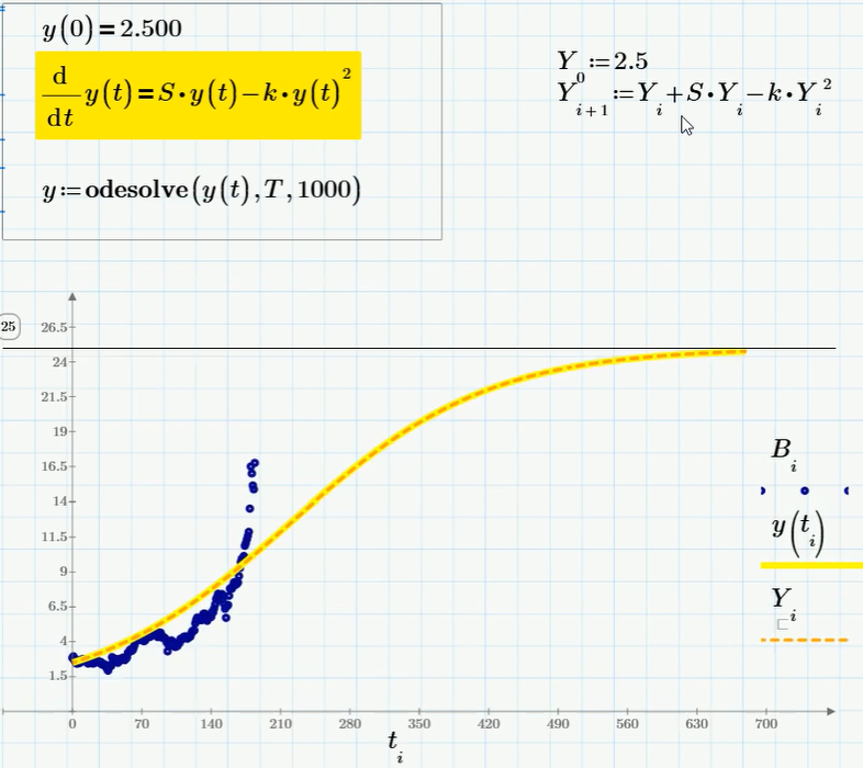
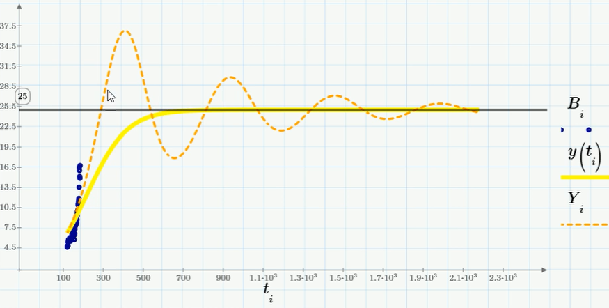
The ODE solution using the built-in Mathcad Prime function is shown as a yellow curve. If you have only the free version of Mathcad Express, then the solution to such a simple ODE as a logistic one can be easily written in the form of an implementation of a difference scheme (a detailed article is devoted to thison Habré). The difference scheme itself contains only two lines of calculations and is written out to the right of the “decision block” circled in the frame. The solution of the ODE using the difference scheme is shown on the same graph in the form of a dashed curve that coincides with the solution y (t). The asymptotic value that y (t) tends to is S / k. Actually, based on these considerations, the coefficient k is selected. We don’t know what it really is (according to the model, bitcoin can grow up to 25, and maybe up to 200, if you take k 10 times less).
The next model is a slight logistical complication, namely, a model of the dynamics of the population subjected to fishing, i.e. uniform withdrawal of a certain share from the population. If we draw an analogy with bitcoin, then this model describes a decrease in the volume of bitcoins due to their sale by speculators (and / or due to a strange commission when exchanging for money, which, as you know, reaches 10-20%). It is also worth considering that the trade (sale of bitcoins) does not start from the very beginning, but from some point, for example, after reaching the equilibrium value S / k. The equation and its solution are as follows:
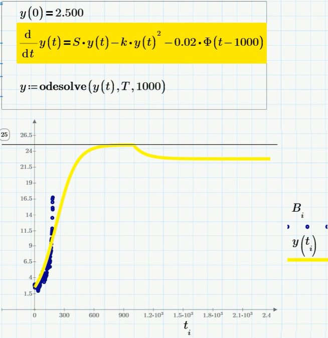
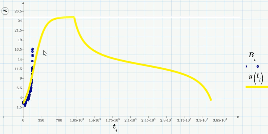
As you can see, fishing causes a certain decrease in the equilibrium rate (in terms of computational biology - population size). But this will happen if only a not very large percentage of the population is exposed to fishing. If the last term in the equation is taken too large (more precisely - more than a certain critical value), then the population will die out instead of the desire for an asymptotic number (and the bitcoin exchange rate, if we draw an analogy, will collapse to zero). The corresponding solution schedule (for the coefficient with the last term of approximately 0.07) is shown in the figure:
Actually, this already describes the financial pyramid quite well: first, rapid exponential growth (the Malthus model) - then saturation and reaching a plateau (the Verhulst model or the logistic model with a small catch) - and in the final, investors' dissatisfaction, panic sales and depreciation to zero. When will this happen? Of course, I will not undertake to predict - perhaps tomorrow, or perhaps in a year.
The last model that is characteristic of financial modeling and which I would like to consider is the “logistic model with delay”. If we want to take into account the presence of speculators who play in a growing market, then the easiest way is to foresee that they buy bitcoin, hold for a while, and then sell. For definiteness, we choose this period of time equal to 120 days. Then the corresponding “logistic equation with delay” will slightly differ from the Verhulst equation y '= S * y - k * y 2namely, to include as the last term not the square y (t), but the product of two values of y (t) taken at two points in time that are 120 days apart. This is also the well-known equation y '(t) = S * y (t) - k * y (t) * y (t-120), which can be solved numerically using the following difference equation in Mathcad Express:
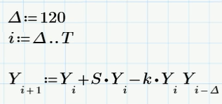
It is noteworthy that the equation with delay has a solution in the form of damped oscillations. And it is possible that before the collapse we will see (or maybe even observe right now?) Such a characteristic correction of the Bitcoin exchange rate. But still, I don’t want to guess, because, once again, this article is a good occasion to show how differential equations are solved in Mathcad and to remind the reader about models from computational biology.
In conclusion, I leave a link to your video, in which the entire sequence of actions in Mathcad for calculating the above models is described in more detail.
Since everything that has been happening lately with bitcoin looks like a pyramid, the models will be appropriate, especially since many colleagues, for example, M. Balandin and V. , devoted their articles to the mathematical apparatus, thanks to MMM . Points . We will pay the main attention, as before, to the methods of calculations in Mathcad, especially in its free version of Mathcad Express , without insisting on the accuracy of the forecast, what the bitcoin exchange rate will be in the near future, and when exactly it will crash.
First of all, it is worth noting that so far, over the past few months, the graph of the Bitcoin exchange rate has strongly resembled exponential growth (see the graph above). Those. it begs the use of an equation of the type y '(t) = S * y (t), the solution of which is an exponential function. To be able to compare experimental data and simulation results in Mathcad, you must first import the source data into a Mathcad document. To how this is done (by the way, import also works in the free version of Mathcad Express) I dedicated a screencast in which I also showed how data can be interpolated and extrapolated using an exponential function. The result of interpolation-extrapolation is shown in the upper graph of the red (according to the data for the last year) and orange (4 months) curves.
In this article, we will calculate several simple well-known models based on ordinary differential equations . They were originally proposed as models of the growth of biological populations (see in more detail, for example, here), and subsequently began to be used to model epidemics, as well as economic phenomena similar to this one. The first model is y '(t) = S * y (t), where y (t) - we consider the bitcoin exchange rate at time t. This world famous model was proposed by Malthus in 1798 in his classic work On the Law of Population Growth. If we draw an analogy with the dynamics of the population, or rather, with the spread of the epidemic, then y (t) would be more adequate to consider the total capitalization of Bitcoin, i.e. value of the current rate multiplied by the number of bitcoins. But since the number of bitcoins has changed little over the year (and it has increased due to mining), for simplicity and clarity, y (t) can be considered the current rate.
We turn now to the next model - the Verhulst equation y '= S * y - k * y 2, in which the last term describes the attenuation of the epidemic due to resource limitations. Accordingly, let's look at this example how in mathcad prime and mathcad express it is possible to solve ordinary differential equations (hereinafter ODE). In the fully functional version of mathcad prime, a “solution block” is used for this, in which the initial condition is written, the differential equation itself (it is highlighted in yellow), as well as the built-in mathcad prime function that solves it.
The ODE solution using the built-in Mathcad Prime function is shown as a yellow curve. If you have only the free version of Mathcad Express, then the solution to such a simple ODE as a logistic one can be easily written in the form of an implementation of a difference scheme (a detailed article is devoted to thison Habré). The difference scheme itself contains only two lines of calculations and is written out to the right of the “decision block” circled in the frame. The solution of the ODE using the difference scheme is shown on the same graph in the form of a dashed curve that coincides with the solution y (t). The asymptotic value that y (t) tends to is S / k. Actually, based on these considerations, the coefficient k is selected. We don’t know what it really is (according to the model, bitcoin can grow up to 25, and maybe up to 200, if you take k 10 times less).
The next model is a slight logistical complication, namely, a model of the dynamics of the population subjected to fishing, i.e. uniform withdrawal of a certain share from the population. If we draw an analogy with bitcoin, then this model describes a decrease in the volume of bitcoins due to their sale by speculators (and / or due to a strange commission when exchanging for money, which, as you know, reaches 10-20%). It is also worth considering that the trade (sale of bitcoins) does not start from the very beginning, but from some point, for example, after reaching the equilibrium value S / k. The equation and its solution are as follows:
As you can see, fishing causes a certain decrease in the equilibrium rate (in terms of computational biology - population size). But this will happen if only a not very large percentage of the population is exposed to fishing. If the last term in the equation is taken too large (more precisely - more than a certain critical value), then the population will die out instead of the desire for an asymptotic number (and the bitcoin exchange rate, if we draw an analogy, will collapse to zero). The corresponding solution schedule (for the coefficient with the last term of approximately 0.07) is shown in the figure:
Actually, this already describes the financial pyramid quite well: first, rapid exponential growth (the Malthus model) - then saturation and reaching a plateau (the Verhulst model or the logistic model with a small catch) - and in the final, investors' dissatisfaction, panic sales and depreciation to zero. When will this happen? Of course, I will not undertake to predict - perhaps tomorrow, or perhaps in a year.
The last model that is characteristic of financial modeling and which I would like to consider is the “logistic model with delay”. If we want to take into account the presence of speculators who play in a growing market, then the easiest way is to foresee that they buy bitcoin, hold for a while, and then sell. For definiteness, we choose this period of time equal to 120 days. Then the corresponding “logistic equation with delay” will slightly differ from the Verhulst equation y '= S * y - k * y 2namely, to include as the last term not the square y (t), but the product of two values of y (t) taken at two points in time that are 120 days apart. This is also the well-known equation y '(t) = S * y (t) - k * y (t) * y (t-120), which can be solved numerically using the following difference equation in Mathcad Express:
It is noteworthy that the equation with delay has a solution in the form of damped oscillations. And it is possible that before the collapse we will see (or maybe even observe right now?) Such a characteristic correction of the Bitcoin exchange rate. But still, I don’t want to guess, because, once again, this article is a good occasion to show how differential equations are solved in Mathcad and to remind the reader about models from computational biology.
In conclusion, I leave a link to your video, in which the entire sequence of actions in Mathcad for calculating the above models is described in more detail.