Interpolation polynomial on arbitrary functions

Introduction

Greetings, dear readers! Today I propose to reflect on the following task:

Given$$ pairs of points on the plane $$. Everything$$are different. Need to find polynomial$$ such that $$where $$

Translating into Russian we have: Ivan made $$points on the plane, and Mary, having this information, should come up with a function that (at least) will go through all these points. In the framework of the current article, our task is to help Mary in a roundabout way.

“Why in a roundabout way?” You ask. The answer is traditional: this article is a continuation of a series of amateurish articles about mathematics, the purpose of which is to popularize the mathematical world.

Process

To begin with, it is worth noting that a certain number of interpolation polynomials already, of course, exist. These polynomials are just designed to solve the desired problem. Among them are especially known such as the Lagrange and Newton polynomials .

It is also necessary to clarify what “arbitrary functions” are (the term comes from the title of the current article). By them is meant any unary function whose result is a bijective mapping of the argument.

In the framework of the article, I propose to take the decimal logarithm for such a function$$ and the following points:

$$

Representing them on the plane, something like this should turn out:


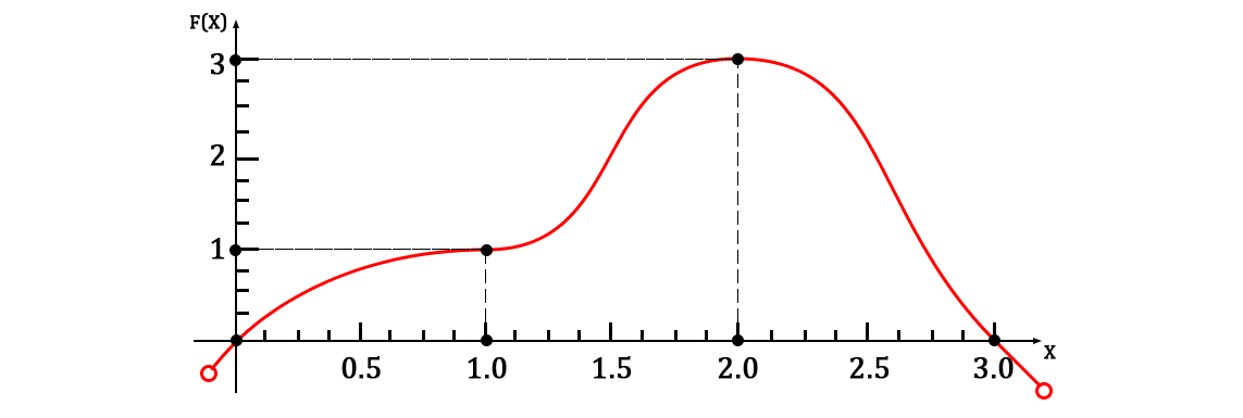
It is easy to notice that now the number of pairs of points is equal to$$.

When solving this problem, a certain system of equations comes to mind, where the number of linearly independent lines is$$. What kind of system of equations is this?

Let's try to write a function as a sum of decimal logarithms with coefficients (so that the number of coefficients is equal to$$):

$$

Arguments for $$different to avoid linear dependence of strings in the future (you can think of others). And also, considering that the domain of definition of the function is at least$$ (based on points specified by the condition), we thus ensure the existence of a range of values ​​for the function $$in this area of ​​definition.

Since we know$$ pairs of points, then we turn to them in order to construct the following trivial system:

$$

The triviality of the system is that we simply find such $$that will satisfy the entire set of conditions.

Actually solving this system relatively$$ we get the following solution:

$$

On this, the task naturally comes to an end, it remains only to write it into a single function:

$$

She, of course, will go through a given set of points. A graph of the function will look like this:


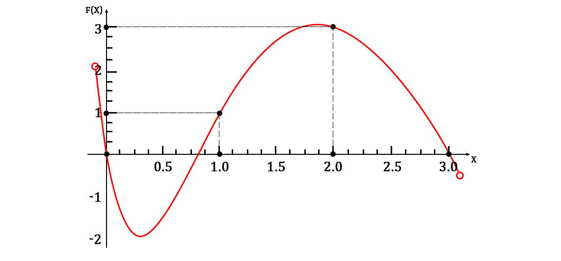
Also, for the sake of clarity, we can give an approximated system of solutions:

$$

Then the approximated form of the function will be as follows:

$$

Of course, no one says that the resulting function will be minimal (the same Lagrange polynomial will give a shorter form). However, this method allows you to express a function through a set of arbitrary functions (though, bearing in mind the restrictions specified above in the article).

Various examples

For dessert, we similarly construct a function in radicals :

$$

We compose a system of equations for finding the coefficients:

$$

Her solution is unique and looks as follows:

$$

Then the finished function is as follows:

$$

Which, in combination, is the Lagrange polynomial for a given set of points (since it implicitly implements the radical form of the algorithm from the article). The graph on the area of ​​the given points looks like this:



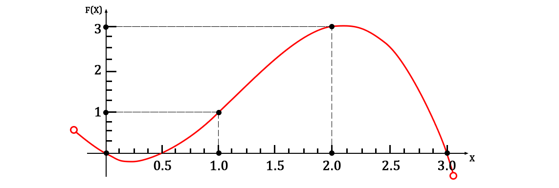
The most interesting in this story is that arbitrary functions for constructing the final function can and should be combined. In other words, a function can be built immediately on radicals and logarithms, or maybe on something else (exponential functions, factorials, etc.). If only the obtained set of functions provided linear independence of the rows in the selection of coefficients. In general form for given$$ pairs of points it looks like this:

$$

Where $$ - the coefficients to be found through the system of equations (SLAE), and $$- some functions that provide linear independence in finding the coefficients.

And then - according to the algorithm above, everything is exactly the same. Not forgetting that$$must be defined at conditionally specified points.

For example, you can show a function consisting of completely different basic functions:

$$

In order to satisfy a given set of points, the coefficients will then be the following (found strictly according to the algorithm from the article):

$$

And the function itself will be like this:

$$

The graph will look almost the same as the previous one (in the area of ​​the given points).
If you want a more “smooth” schedule, then you can look in the direction of the factorial form, for example this:

$$

Find the coefficients:

$\$\$\; display\; \$\$\; \backslash \; begin\; \{cases\}\; \backslash \; displaystyle\; \{2a\; +\; b\; +\; c\; +\; d\; =\; 0\; \backslash \backslash \; 6a\; +\; 2b\; +\; c\; +\; d\; =\; 1\; \backslash \backslash \; 24a\; +\; 6b\; +\; 2c\; +\; d\; =\; 3\; \backslash \backslash \; 120a\; +\; 24b\; +\; 6c\; +\; d\; =\; 0\}\; \backslash \; end\; \{cases\}\; \backslash \; Rightarrow\; \backslash \; begin\; \{cases\}\; \backslash \; displaystyle\; \{a\; =\; -13/16\; \backslash \backslash \; b\; =\; 17/4\; \backslash \backslash \; c\; =\; -3/8\; \backslash \backslash \; d\; =\; -9\; /\; 4\; \}\; \backslash \; end\; \{cases\}\; \$\$\; display\; \$\$$

Substitute these in the finished function:

$$

And also enjoy a very good schedule:

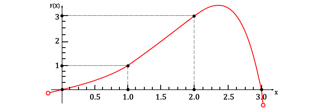
Why is this needed?

Yes, at least in order to imagine a bunch of ropes tightened with plastic clamps :)

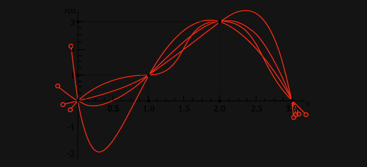
( * Here we just laid all the charts on top of each other )

That's all for the current article, I recommend playing on your own.

All the best,
Peter was with you.