Bird Detection with the Azure ML Workbench
Have you ever thought that biologists, among other things, have a number of important tasks? They need to analyze huge amounts of information to track population dynamics, identify rare species, and assess impact. Under the cut, we want to tell you about a project to identify red-footed kittiwakes in photographs taken using security cameras. You'll learn more about data markup, Azure Machine Learning Workbench model training using the Microsoft Cognitive Toolkit (CNTK) and Tensorflow, and deploying a prediction web service.
This article is a translation of Bird Detection with Azure ML Workbench .
The video below is provided Abram Fleischmann (State University in San Jose) and by Conservation Metrics, Inc . It captures the natural habitat of the red-footed duckweed - a species of bird for which it is necessary to develop a means of detection. Using various equipment, including climbing equipment, biologists install cameras on the rocks to take pictures both day and night.
To train the model, photographs were used, and image markup was performed using the Visual Object Tagging Tool (VOTT) . The markup of the data took about 20 hours, during which time about 12,000 bounding boxes were noted.

Tagged data is available in the repository on GitHub .
These data were collected by Dr. Rachel Orben (University of Oregon), Abram Fleishman (State University of San Jose) and Conservation Metrics, Inc. as part of a major project to study the early nesting period of the red-footed warrior, determine the influence of the factor of food availability and analyze the non-breeding period in the Bering Sea (Alaska).
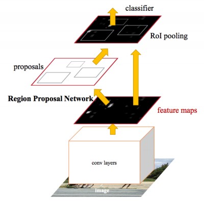
For more information on object detection technologies, see the blog post on convolutional neural networks (CNNs) . Faster R-CNN (Region proposals with Convolutional Neural Network) - a relatively new approach (the first document on this method was published in 2015). It is widely used by the machine learning community and is now embedded in the most popular deep neural network (DNN) frameworks, including PyTorch, CNTK, Tensorflow, Caffe and others.
In this article, we will look at the Faster R-CNN algorithm for detecting objects using the CNTK and Tensorflow frameworks.
We used the recently announced Azure Machine Learning Workbench platform to train the model and create forecasting web services . It is a set of analytical tools and allows data specialists to prepare data, run machine learning experiments and deploy models in a cloud environment (see the documentation in the “ Installation and Setup ” section).
Since we have to work with images, we used the MNIST handwritten numeral classification model at CNTK and Tensorflow, a tool to start the experiment.

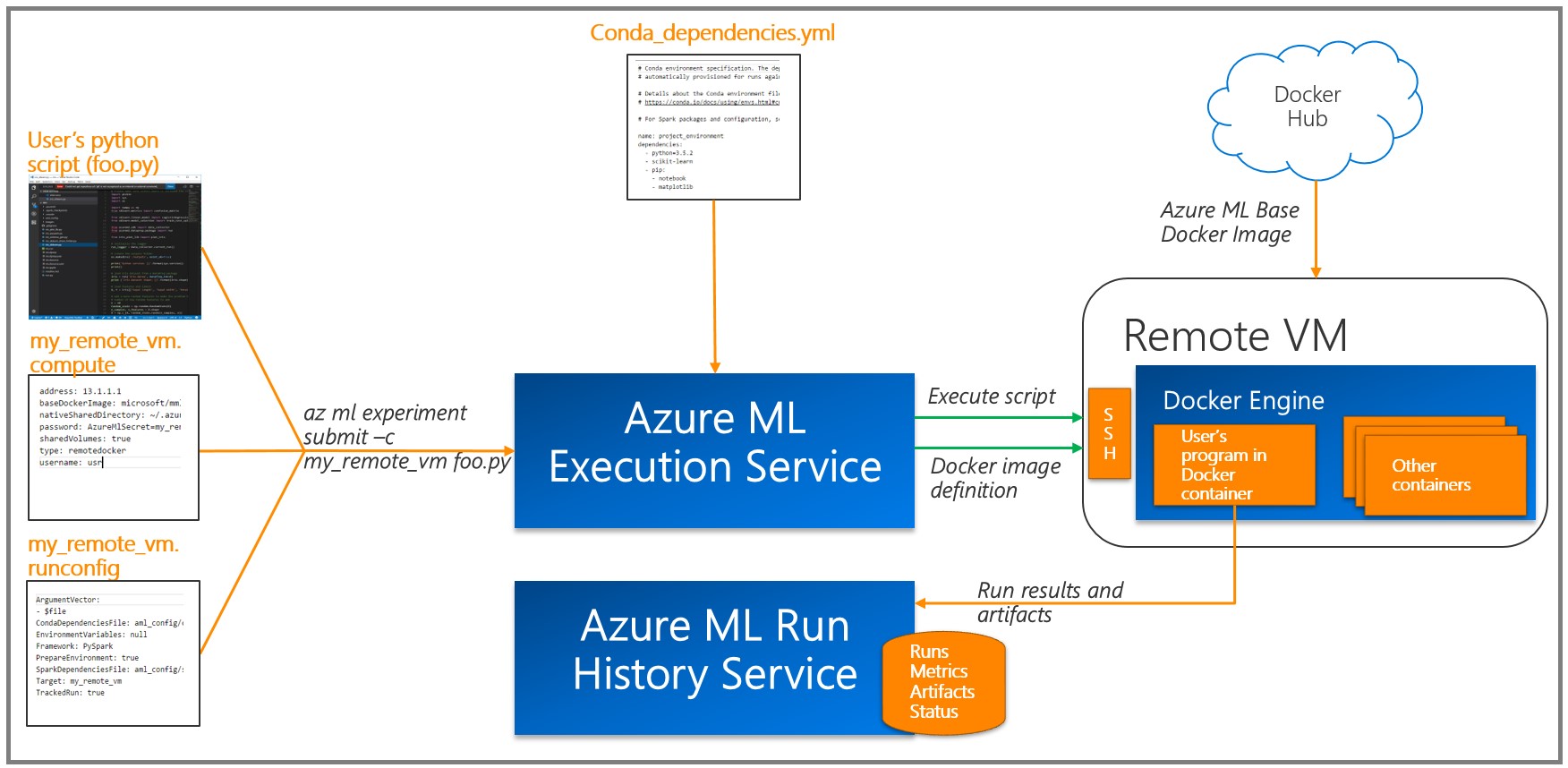
As a rule, deep neural network (DNN) training is performed efficiently using a graphics processing unit (GPU), which significantly speeds up a number of matrix operations. To train the models, we deployed virtual machines to process and analyze data from the GPU and used the remote Docker runtime available in the Azure ML Workbench (see the " Details " section and additional information about target platforms ).
Azure ML writes the results of each task (experiment) to the execution log. Since various combinations of model parameters were used in the experiments, this feature turned out to be very useful: the available visualization tools help to choose the model with the best performance. Note that you must add the tool using the Azure ML Logging API to the training / assessment code in order to track the metrics you need (for example, classification accuracy).
We used the VOTT utility (available for Windows and MacOS) to markup and export data to CNTK and Tensorflow Pascal formats, respectively.
This is a tool with a convenient interface for identification, which allows you to mark the desired area on images and videos. To work with it, you need to collect images in a folder, then run VOTT, specify a set of image data and go to marking areas.

When finished, click Object Detection, then Export Tags to export to CNTK and Tensorflow.
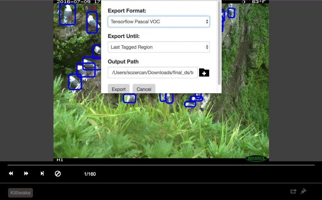
In Tensorflow, the export format is VOC Pascal, so we converted the data to TFRecords for use in training and evaluation. We will describe in more detail below.
As stated in the previous section, in the bird detection model we used the popular Faster R-CNN algorithm . In this section, we will focus on two aspects of our approach:
Setting hyperparameters is the main stage in the process of building ready-to-use machine learning models (or deep learning), provided that the first draft of the model showed good results. The problem here is the efficient implementation and simplification of the process through the Azure ML Workbench.
To configure the parameters, a large number of training experiments are required, which usually takes a very long time. One of the approaches is based on training on a powerful local computer or cluster. However, our approach is aimed at learning in the cloud using Docker containers on remote (virtual) machines. The main advantage is that now we can issue the required number of containers for parallel settings. In accordance withWith this documentation for Azure ML, you need to register each virtual machine as a calculation target for the experiment. Please note that there are restrictions on password characters, for example, using the “*” character in a password will cause an error.
After the command will create a file
We used Azure Storage to store training data, pre-trained models, and model breakpoints. Storage credentials are listed as
Now we can execute the command to start the preparation of the machine.
Then we will train the model for detecting objects.
With Azure ML and Workbench, you can easily record hyperparameters and other performance metrics by running multiple containers at the same time (for more information, see the " Logging Information " section of the documentation).
The first approach to try is to use different pre-trained basic models. At the time of this writing, the CNTK Faster R-CNN API method supported two basic models: AlexNet and VGG16 . We can use these trained models to highlight image features. Although these basic models were trained on other datasets such as ImageNet, at a low and medium level, the features of the images are the same in different applications and, therefore, publicly available. This phenomenon is known as learning transfer.
AlexNet has five convolutional CONV layers, while VGG16 has twelve. The number of trained parameters in VGG16 is 138 million, which exceeds AlexNet almost three times; here we used the VGG16 as the base model. The following are VGG16 hyperparameters optimized to achieve better performance on the scorecard.
In Detection / FasterRCNN / FasterRCNN_config.py:
In Detection / utils / configs / VGG16_config.py:
Azure ML Workbench greatly simplifies the visualization and comparison of different parameter configurations.

For implementation instructions, see the GitHub repository .
Google recently introduced a powerful set of APIs for object discovery. We used their documentation on training animal recognition tools using the Google Cloud Machine Learning Engine , which was an inspiration for us in developing a project to train the model for detection of milkworms on the Azure ML Workbench. The Tensorflow Object Detection API contains many pre-trained models on the COCO dataset . In our experiments, we used ResNet-101 ( deep residual network , 101 layers) as the base model and applied the configurationsanimal recognition example to start setting up object detection training.
This repository contains scripts used to train object discovery models through Azure ML Workbench and Tensorflow.
Step 1. Prepare the data in TF Records format, which is required for the Tensorflow Object Detection API. For this approach, the standard output of the VOTT tool must be converted . See the create_pascal_tf_record.py generic converter for more details .
Step 2. Create a Tensorflow Object Detection and Slim code package for further installation in the Docker image, which is used for experimentation. The following are the steps from the Tensorflow object discovery documentation :
Then move the created tarballs to a place accessible for experimentation (for example, in blob storage) and place the link in
Step 3. In the experiment script add import.
Then call the training procedure in your code using the training_module (_) function.
Detection of the Tensorflow Object Detection API involves starting training and evaluation (checking the model’s current performance) by running two separate commands from the command line. When starting several experiments, it is advisable to periodically run an assessment (for example, every 100 iterations) to analyze the model's ability to recognize objects in hidden data.
In the case of Tensorflow Object Detection AP, we added train_eval.py , which demonstrates the approach to continuous learning and evaluation.
To establish several model hyperparameters and evaluate their impact on the model, we divided the data into training, validation (customizable) and test sets : 160 images, 54 and 55 images, respectively.
The Tensorflow Object Detection Framework provides users with various parameter settings, allowing them to choose the best option for a particular data set.
In this exercise, we will do a few runs and see which one provides the best model performance. As the target metric, we will use the accuracy of object detection, which is usually defined as mAP (Mean Average Precision, averaged value of average accuracy). In each run, we use
TensorBoard is a powerful tool for debugging and visualizing deep neural networks (DNNs). The Tensorflow Object Detection API already provides summary metrics for accuracy. In this project, we integrated the Tensorflow summary events used by TensorBoard for visualization with the Azure ML Workbench.
See the results_logger.py code for more details .
Here is an analysis of several training runs conducted using the Azure ML Workbench experimentation infrastructure.
Run No. 1 uses the method of stochastic gradient descent, data augmentation is disabled (for a review of the possibilities of gradient optimization, see this blog entry).
The execution log in the Azure ML Workbench provides detailed information about each run:
In this case, we see that the maximum mAP value was 93.37% at about 3,500 iterations. Accordingly, the model is retrained for the training data, and the performance on the test set begins to decline.
Run No. 2uses advanced Adam optimization algorithm. All other parameters are the same.

Here, the mAP value of 93.6% is achieved much faster than in run No. 1. Apparently, the retraining of the model occurs much earlier, since the accuracy value on the evaluation set is rapidly decreasing.
Run No. 3 adds data augmentation to the training configuration. For subsequent runs, we will leave the Adam optimization algorithm.
Random horizontal display of images allowed to improve mAP indicators from 93.6 in run No. 2 to 94.2%. More iterations are also required to retrain the model.
Run No. 4 contains more data augmentation options.
Interesting results are presented below:

Despite the fact that the mAP value is not maximum (91.1%), after 7,000 iterations, retraining does not occur. In this case, it is logical to continue training this model in order to understand whether it is possible to increase the value of mAP.
Here is a brief overview of the learning process using the Azure ML Workbench:

Azure ML Workbench allows users to compare runs in parallel (runs No. 1, 3 and 4 are shown below):

In addition, we can build graphs with the assessment results on the desired image (s) and also use them when comparing values. TensorBoard events already contain all the necessary data.
Thus, the detection of objects based on ResNet allows us to achieve better results even on small data sets. Azure ML Workbench has a useful infrastructure that provides a single area for performing experiments and comparing results.
After developing a model for object detection and classification with sufficient performance, we proceed to deploy the model in the form of a hosted web service in such a way as to be able to connect to the bird watching application. We’ll show you how to do this with the built-in Azure ML tools and how to perform a custom deployment.
Azure ML provides enhanced support for model operationalization on a local computer or Azure cloud platform.
Before deploying the model as a web service, you must run SSH on the VM you are using.
In this example, we use a VM to process and analyze the Azure data on which the Azure CLI is installed. If using a different VM, install the Azure CLI using:
Log in using:
First, register your environment provider with:
When deploying a web service on a local computer, you first need to prepare the environment:
This step allows you to create a resource group, storage account, Azure Container Registry (ACR), and Application Insights account.
Set up the environment as shown:
Create a model management account:
Now you are ready to deploy the model! You can create a service using:
Please note that nvidia-docker is not currently available for forecasting. Be sure to change Conda dependencies to remove any GPU related links, such as tensorflow-gpu.
After you deploy the service, you can view information about how to use the web service with:
For example, you can test the service with the command
Another way to deploy a predictive web service is to create your own instance of the Sanic web server . Sanic is a Python 3.5+ web server similar to Flask, which allows you to create and run web applications. We can use the model trained using CNTK and Faster R-CNN in the previous section to perform prediction to identify the location of the bird in the image.
First you need to create the Sanic web application. You can use the following code snippet (and app.py ) to create a web application and determine where it will run on the server. For each API you need, you can specify routes, HTTP methods, and methods for processing each request.
Once the web application is defined, it is necessary to implement the logic in order to use the image path and return the predicted results to the user.
Using predict.py , we first load the image for which we need to build a forecast, then evaluate it relative to a previously trained model to return the predicted data to JSON.
The returned JSON is an array of predicted labels and bounding boxes for each bird found in the image:
Now that we have implemented the forecasting logic and the web service, we can host the application on the server. We will use Docker so that the deployment dependencies and the process itself are simple and reproducible.
Create a Docker image using the Dockerfile so that you can run the application as a Docker container:
Now we can build the Docker image by running:
When the Docker cmcntk image is available locally, we will be able to launch its instances as containers. Using the command below, we connect the volume node to cmcntk in the container to ensure data stability (this refers to the previous step when we trained the model). Then we map the port of node 80 to the port of container 80 and run the last Docker cncntk image.
Now we can test the web service using the curl command:
Now our services are running. What's next? How does a customer interact with them? How to unify them under one API? During our work with Conservation Metrics, we created the application as an experimental solution to complete the entire classification process.
We know what operations are needed for the application, but due to a number of limitations of current services there may be interaction problems. Including:
To create a universal API endpoint, configure the Azure API Management Service . This way we can configure and expose CORS-enabled endpoints for our APIs.
Beginning of work:
Configuration:

Initial API configuration:

After preparing, go to the API. Click the “+ Add API” button, then select the “Blank API” option. Configure the API so that the Web service URL is an API on an external server, the suffix API is represented by a suffix that will be added to the URL for managing the API, and on the Products tab, the required type of API product under which you want to register this final point.
In the created API, configure the “Inbound processing” item using the “Code View” item and set the following values for the policies (to activate CORS support for all external URLs):
You can work with the Suffix URL API, which you configured in the API control section, as when directly checking the connection on our API.
Although the examples are from the old Azure Management Portal , you might want to check out the more detailed getting started guide (API Management Services and CORS Policy).
Our sample web client application performs the following actions:
GitHub code .
The only difference between checking the connection of the API management services from the "native" APIs is that in all requests you need to add an additional Ocp-Apim-Subscription-Key header. This subscription key is bound to an API management product that contains the specified API endpoints.
To get a subscription key:
In the same sample application, add this subscription key as a value for the attached header
Now you can check the connection of services with the image and get a list of returned bounding boxes.
The basic use case is to draw frames on the image. One easy way to do this on the web client is to display the image and apply the frame overlay using:
This code will be transferred to the canvas, it is almost indicated as in the figure below:

Now you can interact with the trained model and demonstration results of forecasting. See the code on this GitHub repository for more details .
In this article, we examined a comprehensive process for detecting objects, including:
We remind you that you can try Azure for free .
This article is a translation of Bird Detection with Azure ML Workbench .
Data
The video below is provided Abram Fleischmann (State University in San Jose) and by Conservation Metrics, Inc . It captures the natural habitat of the red-footed duckweed - a species of bird for which it is necessary to develop a means of detection. Using various equipment, including climbing equipment, biologists install cameras on the rocks to take pictures both day and night.
To train the model, photographs were used, and image markup was performed using the Visual Object Tagging Tool (VOTT) . The markup of the data took about 20 hours, during which time about 12,000 bounding boxes were noted.
Tagged data is available in the repository on GitHub .
Where is the data from
These data were collected by Dr. Rachel Orben (University of Oregon), Abram Fleishman (State University of San Jose) and Conservation Metrics, Inc. as part of a major project to study the early nesting period of the red-footed warrior, determine the influence of the factor of food availability and analyze the non-breeding period in the Bering Sea (Alaska).
Object Discovery
For more information on object detection technologies, see the blog post on convolutional neural networks (CNNs) . Faster R-CNN (Region proposals with Convolutional Neural Network) - a relatively new approach (the first document on this method was published in 2015). It is widely used by the machine learning community and is now embedded in the most popular deep neural network (DNN) frameworks, including PyTorch, CNTK, Tensorflow, Caffe and others.
In this article, we will look at the Faster R-CNN algorithm for detecting objects using the CNTK and Tensorflow frameworks.
Azure Machine Learning Workbench
We used the recently announced Azure Machine Learning Workbench platform to train the model and create forecasting web services . It is a set of analytical tools and allows data specialists to prepare data, run machine learning experiments and deploy models in a cloud environment (see the documentation in the “ Installation and Setup ” section).
Since we have to work with images, we used the MNIST handwritten numeral classification model at CNTK and Tensorflow, a tool to start the experiment.
As a rule, deep neural network (DNN) training is performed efficiently using a graphics processing unit (GPU), which significantly speeds up a number of matrix operations. To train the models, we deployed virtual machines to process and analyze data from the GPU and used the remote Docker runtime available in the Azure ML Workbench (see the " Details " section and additional information about target platforms ).
Azure ML writes the results of each task (experiment) to the execution log. Since various combinations of model parameters were used in the experiments, this feature turned out to be very useful: the available visualization tools help to choose the model with the best performance. Note that you must add the tool using the Azure ML Logging API to the training / assessment code in order to track the metrics you need (for example, classification accuracy).
Image Layout and Export
We used the VOTT utility (available for Windows and MacOS) to markup and export data to CNTK and Tensorflow Pascal formats, respectively.
This is a tool with a convenient interface for identification, which allows you to mark the desired area on images and videos. To work with it, you need to collect images in a folder, then run VOTT, specify a set of image data and go to marking areas.
When finished, click Object Detection, then Export Tags to export to CNTK and Tensorflow.
In Tensorflow, the export format is VOC Pascal, so we converted the data to TFRecords for use in training and evaluation. We will describe in more detail below.
Training Bird Detection Model Using CNTK
As stated in the previous section, in the bird detection model we used the popular Faster R-CNN algorithm . In this section, we will focus on two aspects of our approach:
- Use Azure ML Workbench to start learning on remote VMs.
- Configure hyperparameters through the Azure ML Workbench.
Using Azure ML Workbench to train on a remote VM
Setting hyperparameters is the main stage in the process of building ready-to-use machine learning models (or deep learning), provided that the first draft of the model showed good results. The problem here is the efficient implementation and simplification of the process through the Azure ML Workbench.
To configure the parameters, a large number of training experiments are required, which usually takes a very long time. One of the approaches is based on training on a powerful local computer or cluster. However, our approach is aimed at learning in the cloud using Docker containers on remote (virtual) machines. The main advantage is that now we can issue the required number of containers for parallel settings. In accordance withWith this documentation for Azure ML, you need to register each virtual machine as a calculation target for the experiment. Please note that there are restrictions on password characters, for example, using the “*” character in a password will cause an error.
az ml computetarget attach --name "my_dsvm" --address "my_dsvm_ip_address" --username "my_name" --password "my_password" --type remotedockerAfter the command will create a file
myvm.computeand myvm.rucomfigfolder aml_config. Since our task is more suitable for a GPU machine, the following changes need to be made:At myvm.compute
baseDockerImage: microsoft/mmlspark:plus-gpu-0.7.91
nvidiaDocker: true
In myvm.runconfig
EnvironmentVariables:
    "STORAGE_ACCOUNT_NAME":
    "STORAGE_ACCOUNT_KEY":
Framework: Python
PrepareEnvironment: true
We used Azure Storage to store training data, pre-trained models, and model breakpoints. Storage credentials are listed as
EnvironmentVariables. Make sure the conda_dependencies.ymlpackages you need are included. Now we can execute the command to start the preparation of the machine.
az ml experiment –c prepare myvmThen we will train the model for detecting objects.
az ml experiment submit –c Detection/FasterRCNN/run_faster_rcnn.py
..
..
..
Evaluating Faster R-CNN model for 53 images.
Number of rois before non-maximum suppression: 8099
Number of rois  after non-maximum suppression: 1871
AP for       Kittiwake = 0.7544
Mean AP = 0.7544
Configure Hyperparameters through Azure ML Workbench
With Azure ML and Workbench, you can easily record hyperparameters and other performance metrics by running multiple containers at the same time (for more information, see the " Logging Information " section of the documentation).
The first approach to try is to use different pre-trained basic models. At the time of this writing, the CNTK Faster R-CNN API method supported two basic models: AlexNet and VGG16 . We can use these trained models to highlight image features. Although these basic models were trained on other datasets such as ImageNet, at a low and medium level, the features of the images are the same in different applications and, therefore, publicly available. This phenomenon is known as learning transfer.
AlexNet has five convolutional CONV layers, while VGG16 has twelve. The number of trained parameters in VGG16 is 138 million, which exceeds AlexNet almost three times; here we used the VGG16 as the base model. The following are VGG16 hyperparameters optimized to achieve better performance on the scorecard.
In Detection / FasterRCNN / FasterRCNN_config.py:
# Learning parameters
__C.CNTK.L2_REG_WEIGHT = 0.0005
__C.CNTK.MOMENTUM_PER_MB = 0.9
# The learning rate multiplier for all bias weights
__C.CNTK.BIAS_LR_MULT = 2.0
In Detection / utils / configs / VGG16_config.py:
__C.MODEL.E2E_LR_FACTOR = 1.0
__C.MODEL.RPN_LR_FACTOR = 1.0
__C.MODEL.FRCN_LR_FACTOR = 1.0
Azure ML Workbench greatly simplifies the visualization and comparison of different parameter configurations.
mAP using the base model VGG16
Evaluating Faster R-CNN model for 53 images.
Number of rois before non-maximum suppression: 6998
Number of rois  after non-maximum suppression: 2240
AP for       Kittiwake = 0.8204
Mean AP = 0.8204
For implementation instructions, see the GitHub repository .
Tensorflow Bird Detection Training
Google recently introduced a powerful set of APIs for object discovery. We used their documentation on training animal recognition tools using the Google Cloud Machine Learning Engine , which was an inspiration for us in developing a project to train the model for detection of milkworms on the Azure ML Workbench. The Tensorflow Object Detection API contains many pre-trained models on the COCO dataset . In our experiments, we used ResNet-101 ( deep residual network , 101 layers) as the base model and applied the configurationsanimal recognition example to start setting up object detection training.
This repository contains scripts used to train object discovery models through Azure ML Workbench and Tensorflow.
Training preparation
Step 1. Prepare the data in TF Records format, which is required for the Tensorflow Object Detection API. For this approach, the standard output of the VOTT tool must be converted . See the create_pascal_tf_record.py generic converter for more details .
python create_pascal_tf_record.py
    --label_map_path=/data/pascal_label_map.pbtxt
    --data_dir=/data/
    --output_path=/data/out/pascal_train.record
    --set=train
python create_pascal_tf_record.py
    --label_map_path=/data/pascal_label_map.pbtxt
    --data_dir=/data/
    --output_path=/data/out/pascal_val.record
    --set=val
Step 2. Create a Tensorflow Object Detection and Slim code package for further installation in the Docker image, which is used for experimentation. The following are the steps from the Tensorflow object discovery documentation :
# From tensorflow/models/research/
 python setup.py sdist
 (cd slim && python setup.py sdist)
Then move the created tarballs to a place accessible for experimentation (for example, in blob storage) and place the link in
conda_dependancies.yamlfor the experiment.dependencies:
-python=3.5.2
-tensorflow-gpu
-pip:
#... More dependencies here…
#TF Object Detection
-https:///object_detection-0.1.tar.gz
-https:////slim-0.1.tar.gzStep 3. In the experiment script add import.
from object_detection.train import main as training_moduleThen call the training procedure in your code using the training_module (_) function.
Learning and assessment process
Detection of the Tensorflow Object Detection API involves starting training and evaluation (checking the model’s current performance) by running two separate commands from the command line. When starting several experiments, it is advisable to periodically run an assessment (for example, every 100 iterations) to analyze the model's ability to recognize objects in hidden data.
In the case of Tensorflow Object Detection AP, we added train_eval.py , which demonstrates the approach to continuous learning and evaluation.
 print("Total number of training steps {}".format(train_config.num_steps))
 print("Evaluation will run every {} steps".format(FLAGS.eval_every_n_steps))
 train_config.num_steps = current_step
 while current_step <= total_num_steps:
   print("Training steps # {0}".format(current_step))
   trainer.train(create_input_dict_fn, model_fn, train_config, master, task,
   FLAGS.num_clones, worker_replicas, FLAGS.clone_on_cpu, ps_tasks,
   worker_job_name, is_chief, FLAGS.train_dir)
   tf.reset_default_graph()
   evaluate_step()
   tf.reset_default_graph()
   current_step = current_step + FLAGS.eval_every_n_steps
   train_config.num_steps = current_step
To establish several model hyperparameters and evaluate their impact on the model, we divided the data into training, validation (customizable) and test sets : 160 images, 54 and 55 images, respectively.
Run Comparison
The Tensorflow Object Detection Framework provides users with various parameter settings, allowing them to choose the best option for a particular data set.
In this exercise, we will do a few runs and see which one provides the best model performance. As the target metric, we will use the accuracy of object detection, which is usually defined as mAP (Mean Average Precision, averaged value of average accuracy). In each run, we use
azureml.loggingto obtain information on the maximum mAP and identify training iterations. In addition, we build a “mAP and iteration” graph and then save it to the output folder for display in the Azure ML Workbench.TensorBoard event integration with Azure ML Workbench
TensorBoard is a powerful tool for debugging and visualizing deep neural networks (DNNs). The Tensorflow Object Detection API already provides summary metrics for accuracy. In this project, we integrated the Tensorflow summary events used by TensorBoard for visualization with the Azure ML Workbench.
from tensorboard.backend.event_processing import event_accumulator
from azureml.logging import get_azureml_logger
ea = event_accumulator.EventAccumulator(eval_path, ...)
df = pd.DataFrame(ea.Scalars('Precision/mAP@0.5IOU'))
max_vals = df.loc[df["value"].idxmax()]
#Plot chart of how mAP changers as training progresses
fig = plt.figure(figsize=(6, 5), dpi=75)
 plt.plot(df["step"], df["value"])
 plt.plot(max_vals["step"], max_vals["value"], "g+", mew=2, ms=10)
 fig.savefig("./outputs/mAP.png", bbox_inches='tight')
# Log to AML Workbench best mAP of the run with corresponding iteration N
 run_logger = get_azureml_logger()
 run_logger.log("max_mAP", max_vals["value"])
 run_logger.log("max_mAP_interation#", max_vals["step"])
See the results_logger.py code for more details .
Here is an analysis of several training runs conducted using the Azure ML Workbench experimentation infrastructure.
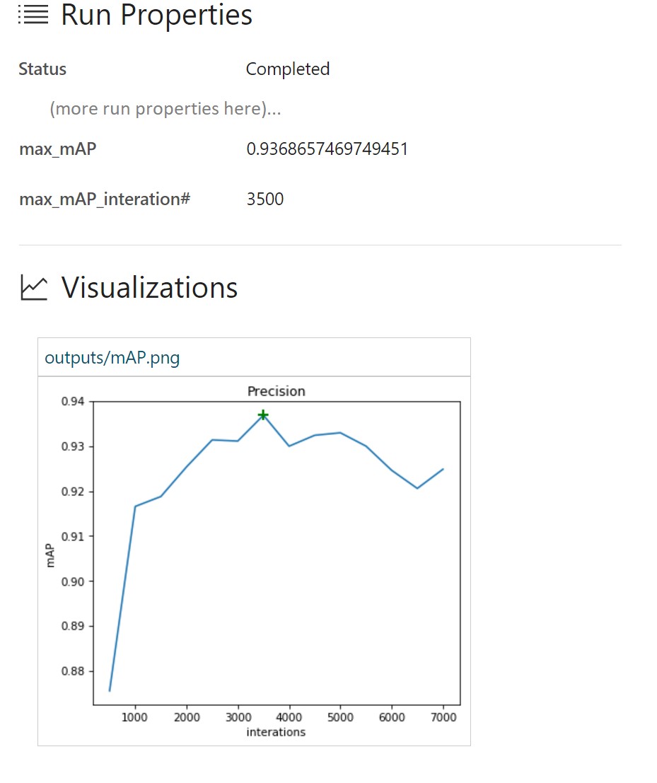
Run No. 1 uses the method of stochastic gradient descent, data augmentation is disabled (for a review of the possibilities of gradient optimization, see this blog entry).
The execution log in the Azure ML Workbench provides detailed information about each run:
In this case, we see that the maximum mAP value was 93.37% at about 3,500 iterations. Accordingly, the model is retrained for the training data, and the performance on the test set begins to decline.
Run No. 2uses advanced Adam optimization algorithm. All other parameters are the same.
Here, the mAP value of 93.6% is achieved much faster than in run No. 1. Apparently, the retraining of the model occurs much earlier, since the accuracy value on the evaluation set is rapidly decreasing.
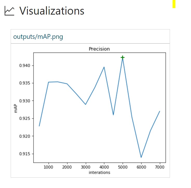
Run No. 3 adds data augmentation to the training configuration. For subsequent runs, we will leave the Adam optimization algorithm.
data_augmentation_options{
  random_horizontal_flip{}
}
Random horizontal display of images allowed to improve mAP indicators from 93.6 in run No. 2 to 94.2%. More iterations are also required to retrain the model.
Run No. 4 contains more data augmentation options.
data_augmentation_options{
  random_horizontal_flip{}
  random_pixel_value_scale{}
  random_crop_image{}
}
Interesting results are presented below:
Despite the fact that the mAP value is not maximum (91.1%), after 7,000 iterations, retraining does not occur. In this case, it is logical to continue training this model in order to understand whether it is possible to increase the value of mAP.
Here is a brief overview of the learning process using the Azure ML Workbench:
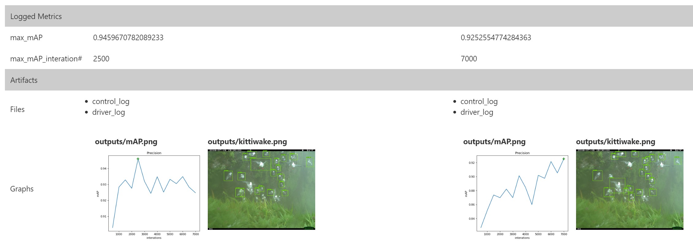
Azure ML Workbench allows users to compare runs in parallel (runs No. 1, 3 and 4 are shown below):
In addition, we can build graphs with the assessment results on the desired image (s) and also use them when comparing values. TensorBoard events already contain all the necessary data.
Thus, the detection of objects based on ResNet allows us to achieve better results even on small data sets. Azure ML Workbench has a useful infrastructure that provides a single area for performing experiments and comparing results.
Deploying Evaluation Web Services
After developing a model for object detection and classification with sufficient performance, we proceed to deploy the model in the form of a hosted web service in such a way as to be able to connect to the bird watching application. We’ll show you how to do this with the built-in Azure ML tools and how to perform a custom deployment.
Web Services Using the Azure ML CLI
Azure ML provides enhanced support for model operationalization on a local computer or Azure cloud platform.
Install Azure ML CLI
Before deploying the model as a web service, you must run SSH on the VM you are using.
ssh @In this example, we use a VM to process and analyze the Azure data on which the Azure CLI is installed. If using a different VM, install the Azure CLI using:
pip install azure-cli
pip install azure-cli-ml
Log in using:
az loginEnvironment preparation
First, register your environment provider with:
az provider register -n Microsoft.MachineLearningComputeWhen deploying a web service on a local computer, you first need to prepare the environment:
az ml env setup -l [Azure region, e.g. eastus2] -n [environment name] -g [resource group]This step allows you to create a resource group, storage account, Azure Container Registry (ACR), and Application Insights account.
Set up the environment as shown:
az ml env set -n [environment name] -g [resource group]Create a model management account:
az ml account modelmanagement create -l [Azure region, e.g. eastus2] -n [your account name] -g [resource group name] --sku-instances [number of instances, e.g. 1] --sku-name [Pricing tier for example S1]Now you are ready to deploy the model! You can create a service using:
az ml service create realtime --model-file [model file/folder path] -f [scoring file e.g. score.py] -n [your service name] -r [runtime for the Docker container e.g. spark-py or python] -c [conda dependencies file for additional python packages]Please note that nvidia-docker is not currently available for forecasting. Be sure to change Conda dependencies to remove any GPU related links, such as tensorflow-gpu.
After you deploy the service, you can view information about how to use the web service with:
az ml service usage realtime -i [your service name]For example, you can test the service with the command
curl:curl -X POST -H "Content-Type:application/json" --data !! YOUR DATA HERE !! http://127.0.0.1:32769/scoreDeploying Evaluation Web Services Alternative
Another way to deploy a predictive web service is to create your own instance of the Sanic web server . Sanic is a Python 3.5+ web server similar to Flask, which allows you to create and run web applications. We can use the model trained using CNTK and Faster R-CNN in the previous section to perform prediction to identify the location of the bird in the image.
First you need to create the Sanic web application. You can use the following code snippet (and app.py ) to create a web application and determine where it will run on the server. For each API you need, you can specify routes, HTTP methods, and methods for processing each request.
app = Sanic(__name__)
 Config.KEEP_ALIVE = False
server = Server()
 server.set_model()
@app.route('/')
 async def test(request):
 return text(server.server_running())
@app.route('/predict', methods=["POST",])
 def post_json(request):
 return json(server.predict(request))
app.run(host= '0.0.0.0', port=80)
 print ('exiting...')
 sys.exit(0)
Once the web application is defined, it is necessary to implement the logic in order to use the image path and return the predicted results to the user.
Using predict.py , we first load the image for which we need to build a forecast, then evaluate it relative to a previously trained model to return the predicted data to JSON.
regressed_rois, cls_probs = evaluate_single_image(eval_model, img_path, cfg)
bboxes, labels, scores = filter_results(regressed_rois, cls_probs, cfg)
The returned JSON is an array of predicted labels and bounding boxes for each bird found in the image:
[{"label": "Kittiwake", "score": "0.963", "box": [246, 414, 285, 466]},...]Now that we have implemented the forecasting logic and the web service, we can host the application on the server. We will use Docker so that the deployment dependencies and the process itself are simple and reproducible.
cd CNTK_faster-rcnn/DetectionCreate a Docker image using the Dockerfile so that you can run the application as a Docker container:
FROM hsienting/dl_az
COPY ./ /app
ADD run.sh /app/
RUN chmod +x /app/run.sh
ENV STORAGE_ACCOUNT_NAME
ENV STORAGE_ACCOUNT_KEY
ENV AZUREML_NATIVE_SHARE_DIRECTORY /cmcntk
ENV TESTIMAGESCONTAINER data
EXPOSE 80
ENTRYPOINT ["/app/run.sh"]
Now we can build the Docker image by running:
docker build -t cmcntk .When the Docker cmcntk image is available locally, we will be able to launch its instances as containers. Using the command below, we connect the volume node to cmcntk in the container to ensure data stability (this refers to the previous step when we trained the model). Then we map the port of node 80 to the port of container 80 and run the last Docker cncntk image.
docker run -v /:/cmcntk -p 80:80 -it cmcntk:latestNow we can test the web service using the curl command:
curl -X POST http://localhost/predict -H 'content-type: application/json'
-d '{"filename": ""}'
Access to services
Now our services are running. What's next? How does a customer interact with them? How to unify them under one API? During our work with Conservation Metrics, we created the application as an experimental solution to complete the entire classification process.
Problem
We know what operations are needed for the application, but due to a number of limitations of current services there may be interaction problems. Including:
- Many services have common functioning goals (output of markup data), but do not have a common endpoint.
- For direct access to these services, the client requires CORS rights (shared access to resources, regardless of the source), which must be managed on all servers / load balancers.
Decision
To create a universal API endpoint, configure the Azure API Management Service . This way we can configure and expose CORS-enabled endpoints for our APIs.
Azure API Management Services
Beginning of work:
- Visit the website https://ms.portal.azure.com/#create/hub
- Search and select “API management”.
- Create and configure your instance.
Configuration:
- Create a new API.
Initial API configuration:
After preparing, go to the API. Click the “+ Add API” button, then select the “Blank API” option. Configure the API so that the Web service URL is an API on an external server, the suffix API is represented by a suffix that will be added to the URL for managing the API, and on the Products tab, the required type of API product under which you want to register this final point.
In the created API, configure the “Inbound processing” item using the “Code View” item and set the following values for the policies (to activate CORS support for all external URLs):
                *
                *
You can work with the Suffix URL API, which you configured in the API control section, as when directly checking the connection on our API.
Although the examples are from the old Azure Management Portal , you might want to check out the more detailed getting started guide (API Management Services and CORS Policy).
Sample application
Our sample web client application performs the following actions:
- Reads data from containers / blobs directly from Azure blob storage.
- Tests the connection between the new Azure API Management Service and images in blob storage.
- Displays returned prediction data (bounding boxes for birds) in the image.
GitHub code .
Verify API Management Service Communications
The only difference between checking the connection of the API management services from the "native" APIs is that in all requests you need to add an additional Ocp-Apim-Subscription-Key header. This subscription key is bound to an API management product that contains the specified API endpoints.
To get a subscription key:
- Go to the "Publisher Portal" API.
- Select a user in the corresponding menu item.
- Record the subscription key you want to use.
In the same sample application, add this subscription key as a value for the attached header
Ocp-Apim-Subscription-Key:exportasyncfunctioncntk(filename) {
return fetch('/tensorflow/', {
method: 'post',
headers: {
Accept: 'application/json',
'Content-Type': 'application/json',
'Cache-Control': 'no-cache',
'Ocp-Apim-Trace': 'true',
'Ocp-Apim-Subscription-Key': ,
},
body: JSON.stringify({
filename,
}),
})
}
data usage
Now you can check the connection of services with the image and get a list of returned bounding boxes.
The basic use case is to draw frames on the image. One easy way to do this on the web client is to display the image and apply the frame overlay using:
<body><canvasid='myCanvas'>canvas><script>const imageUrl = "some image URL";
    cntk(imageUrl).then(labels => {
      const canvas = document.getElementById('myCanvas')
      const image = document.createElement('img');
      image.setAttribute('crossOrigin', 'Anonymous');
      image.onload = () => {
        if (canvas) {
          const canvasWidth = 850;
          const scale = canvasWidth / image.width;
          const canvasHeight = image.height * scale;
          canvas.width = canvasWidth;
          canvas.height = canvasHeight;
          const ctx = canvas.getContext('2d');
          // render image on convas and draw the square labels
          ctx.drawImage(image, 0, 0, canvasWidth, canvasHeight);
          ctx.lineWidth = 5;
          labels.forEach((label) => {
            ctx.strokeStyle = label.color || 'black';
            ctx.strokeRect(label.x, label.y, label.width, label.height);
          });
        }
      };
      image.src = imageUrl;
    });
  script>
body>
html>
This code will be transferred to the canvas, it is almost indicated as in the figure below:
Now you can interact with the trained model and demonstration results of forecasting. See the code on this GitHub repository for more details .
Conclusion
In this article, we examined a comprehensive process for detecting objects, including:
- data markup;
- Training the CNTK / Tensorflow Object Detection Model using Azure ML Workbench
- Comparison of experiment runs in Azure ML Workbench
- операционализацию модели и развертывание веб-службы прогнозирования;
- обзор демонстрационного приложения для построения прогнозов.
Ресурсы
- Проектный репозиторий GitHub.
- Документация по машинному обучению Azure Machine Learning Workbench.
- Репозиторий GitHub: обнаружение объектов с Microsoft Cognitive Toolkit.
- Репозиторий GitHub: обнаружение объектов с Tensorflow Object Detection API.
- Полезные курсы: Analyzing Big Data with Microsoft R (и экзамен), Perform Cloud Data Science with Azure Machine Learning (и экзамен) и Performing Data Engineering on Microsoft HD Insight (и экзамен).
We remind you that you can try Azure for free .