Mixture Density Networks
Hello!
Let's talk about, as you probably already guessed, neural networks and machine learning. From the title, it is clear that Mixture Density Networks will be discussed, then simply MDN, I don’t want to translate the name and leave it as it is. Yes, yes, yes ... it will be a bit boring mathematics and probability theory, but without it, unfortunately, or fortunately, then decide for yourself, it is difficult to imagine the world of machine learning. But I hasten to reassure you, it will be relatively small and it will not be very difficult. And in general it will be possible to skip it, but just look at a small amount of Python and PyTorch code, that's right, we will write the network using PyTorch, as well as various graphs with results. But the most important thing is that there will be an opportunity to understand a bit and understand what the MD network is.
Well, let's start!
Regression
Let's first refresh our knowledge a bit and remember, quite briefly, what a linear regression is .
We have a vector
 we need to predict the value
  which somehow depends on
  using a certain linear model:


 :
:
Of course, the dependence inherent in the nature of data generation may be different and then we need to add some nonlinearity to our model. Solving the regression problem directly for large and real data is also a bad idea, since there is a matrix there
 dimensions
  , and it is still necessary to find its inverse matrix, and it often happens that such a matrix simply does not exist. In this case, various methods based on gradient descent come to our rescue. And non-linearity of models can be implemented in different ways, including using neural networks.
 But now, let's talk not about this, but about the error functions. What is the difference between SE and Log-Likelihood in the case where the data may have a non-linear relationship?
We deal with the zoo, namely: OLS, LS, SE, MSE, RSS
All this is essentially the same, RSS is the residual sum of squares, OLS is the least squares, LS is the least squares, MSE is the mean squared error, SE is squared error. In different sources you can find different names. The essence of this is only one: the square deviation . You can get confused of course, but you get used to it quickly.
It should be noted that the MSE is the average deviation, some average error value for the entire training data set. In practice, MSE is usually used. The formula is no different: - dataset size,
  - model prediction for
  .
.
It should be noted that the MSE is the average deviation, some average error value for the entire training data set. In practice, MSE is usually used. The formula is no different:

- dataset size, - model prediction for .Stop! Likelihood? This is something from the theory of probability. That's right - this is the theory of probability in its purest form. But how can the standard deviation be related to the likelihood function? And as it turns out connected. Associated with finding the maximum likelihood (Maximum Likelihood) and the normal distribution, to be more precise, with its average
 .
. In order to realize that this is the case, let's look again at the square deviation function:


Now, remembering the formula of normal distribution, we get:

 and remove all the constants in the formula (2), just remove it, do not reduce, because finding the minimum of the function does not depend on them. Then see this:
 - for this property it is worth clarifying that this is a natural logarithm and strictly speaking
  . And in general, the logarithm of a function does not change its maximum, and this is the main feature for us. About the connection with Log-Likelihood and Likelihood and why it will be useful to be discussed below, in a small digression. And so, what we did: removed all the constants, and took the logarithm of the likelihood function. They also removed the minus sign, thus turning the Log-Likelihood into the Negative Log-Likelihood (NLL), the connection between them will also be described as a bonus. As a result, we got the NLL function:
 .
. If we use the MSE standard deviation function, we get from this:

 - expected value, - the parameters of the model, we will further denote them as:
  .
. Conclusion: If, in the regression question, we use the LS family as error functions, then in essence we solve the problem of finding the maximum likelihood function in the case when the distribution is Gaussian. And the predicted value
 equal to the average in the normal distribution. And now we know how all this is connected, how probability theory is related (with its likelihood function and normal distribution) and the methods of standard deviation or OLS. More details about this can be found in [2].
 And here is the promised bonus. If we are talking about the links between the various functions of the error, then we will consider (it is not necessary to read):
Relationship between Cross-Entropy, Likelihood, Log-Likelihood and Negative Log-Likelihood
Suppose we have data  , each point belongs to a certain class, for example
  . There is a total
 классов, при этом класс 1 встречается
  раз, класс 2 —
  раз, а класс —
  раз. На этих данных мы обучили некоторую модель . Функция правдоподобия (Likelihood) для нее будет выглядеть так:
где — предсказанная вероятность для класса .
Берем логарифм от функции правдоподобия и получаем Log-Likelihood:![$\hat{y} \in [0, 1]$](https://habrastorage.org/getpro/habr/formulas/a55/cdf/87c/a55cdf87c3da797e8284e2bcd1652b31.svg) лежит в пределах от 0 до 1, исходя из определения вероятности. Следовательно логарифм будет иметь отрицательное значение. И если умножить Log-Likelihood на -1 мы получим функцию Negative Log-Likelihood (NLL):,
лежит в пределах от 0 до 1, исходя из определения вероятности. Следовательно логарифм будет иметь отрицательное значение. И если умножить Log-Likelihood на -1 мы получим функцию Negative Log-Likelihood (NLL):,  , то получим: равна:
  . Отсюда получаем:
 то получим:
 (бинарная классификация) получим формулу для binary cross entropy (так же можно встретить всем известное название Log-Loss):
Пример. Рассмотрим бинарную классификацию. У нас есть значения классов:
Реальная вероятность для класса 0 равна
  , для класса 1 равна
  . Пусть у нас есть бинарный классификатор который предсказывает вероятность класса 0 для каждого примера, соответственно для класса 1 вероятность равна
  . Построим график значений функции Log-Loss для разных предсказаний :
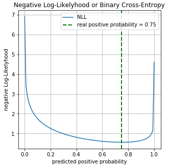
На графике можно увидеть что минимум функции Log-Loss соответствует точке 0.75, т.е. если бы наша модель полностью «выучила» распределение исходных данных, .
.
, each point belongs to a certain class, for example . There is a total классов, при этом класс 1 встречается раз, класс 2 — раз, а класс — раз. На этих данных мы обучили некоторую модель . Функция правдоподобия (Likelihood) для нее будет выглядеть так:

где
— предсказанная вероятность для класса .Берем логарифм от функции правдоподобия и получаем Log-Likelihood:

лежит в пределах от 0 до 1, исходя из определения вероятности. Следовательно логарифм будет иметь отрицательное значение. И если умножить Log-Likelihood на -1 мы получим функцию Negative Log-Likelihood (NLL):
, , то получим:
равна: . Отсюда получаем:
то получим:
(бинарная классификация) получим формулу для binary cross entropy (так же можно встретить всем известное название Log-Loss):
Пример. Рассмотрим бинарную классификацию. У нас есть значения классов:
y = np.array([0, 1, 1, 1, 1, 0, 1, 1]).astype(np.float32)Реальная вероятность
для класса 0 равна , для класса 1 равна . Пусть у нас есть бинарный классификатор который предсказывает вероятность класса 0 для каждого примера, соответственно для класса 1 вероятность равна . Построим график значений функции Log-Loss для разных предсказаний :На графике можно увидеть что минимум функции Log-Loss соответствует точке 0.75, т.е. если бы наша модель полностью «выучила» распределение исходных данных,
.Regression using neural networks
Here we come to the more interesting, to practice. Let's see how you can solve the regression problem using neural networks (neural networks). We will implement everything in the Python programming language; to create a network, we use the PyTorch deep learning library.
Source data generation
Input data
 let's generate using uniform distribution (uniform distribution), we will take an interval from-15 to 15,
 ![$ \ mathbf {X} \ in U [-15, 15] $](https://habrastorage.org/getpro/habr/formulas/12f/bde/d85/12fbded85e3fdc57719df4497a0a4a02.svg) . Points
. Points get using the equation:
 - vector noise dimension obtained using the normal distribution with parameters:
  .
.Data generation
N = 3000# размер данных
IN_DIM = 1
OUT_DIM = IN_DIM
x = np.random.uniform(-15., 15., (IN_DIM, N)).T.astype(np.float32)
noise = np.random.normal(size=(N, 1)).astype(np.float32)
y = 0.5*x+ 8.*np.sin(0.3*x) + noise # формула 3
x_train, x_test, y_train, y_test = train_test_split(x, y) #разобьем на тренировочные и тестовые данные
Graph of the data.
Network building
Create a regular forward distribution network (feed forward neural network or FFNN).
Build FFNN
classNet(nn.Module):def__init__(self, input_dim=IN_DIM, out_dim=OUT_DIM, layer_size=40):
        super(Net, self).__init__()
        self.fc = nn.Linear(input_dim, layer_size)
        self.logit = nn.Linear(layer_size, out_dim)
    defforward(self, x):
        x = F.tanh(self.fc(x)) # формула 4
        x = self.logit(x)
        return x
Our network consists of one hidden layer with the dimension of 40 neurons and with the activation function - the hyperbolic tangent:

Training and getting results
We’ll use AdamOptimizer as an optimizer. Number of learning epochs = 2000, learning rate (learning rate or lr) = 0.1.
FFNN training
deftrain(net, x_train, y_train, x_test, y_test, epoches=2000, lr=0.1):
    criterion = nn.MSELoss()
    optimizer = optim.Adam(net.parameters(), lr=lr)
    N_EPOCHES = epoches
    BS = 1500
    n_batches = int(np.ceil(x_train.shape[0] / BS))
    train_losses = []
    test_losses = []
    for i in range(N_EPOCHES):
        for bi in range(n_batches):
            x_batch, y_batch = fetch_batch(x_train, y_train, bi, BS)
            x_train_var = Variable(torch.from_numpy(x_batch))
            y_train_var = Variable(torch.from_numpy(y_batch))
            optimizer.zero_grad()
            outputs = net(x_train_var)
            loss = criterion(outputs, y_train_var)
            loss.backward()
            optimizer.step()
        with torch.no_grad():
            x_test_var = Variable(torch.from_numpy(x_test))
            y_test_var = Variable(torch.from_numpy(y_test))
            outputs = net(x_test_var)
            test_loss = criterion(outputs, y_test_var)
            test_losses.append(test_loss.item())
            train_losses.append(loss.item())
            if i%100 == 0:
                sys.stdout.write('\r Iter: %d, test loss: %.5f, train loss: %.5f'
                                 %(i, test_loss.item(), loss.item()))
                sys.stdout.flush()
    return train_losses, test_losses
net = Net()
train_losses, test_losses = train(net, x_train, y_train, x_test, y_test)
Now look at the learning outcomes.
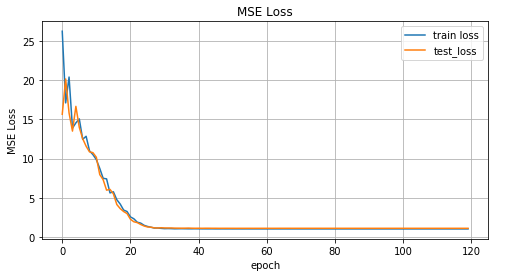
The graph of the MSE function values versus the learning iteration, the graph of the values for the training data and the test data.
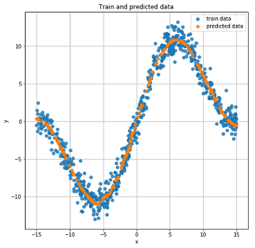
Real and predicted results on test data.
Inverted data
Complicate the task and invert the data.
Invert data
x_train_inv = y_train
y_train_inv = x_train
x_test_inv = y_train
y_test_inv = x_train
Inverted data graph.
To predict
 let's use the direct distribution network from the previous section and see how it handles it.
inv_train_losses, inv_test_losses = train(net, x_train_inv, y_train_inv, x_test_inv, y_test_inv)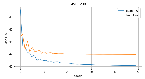
The graph of the MSE function values versus the learning iteration, the graph of the values for the training data and the test data.
Real and predicted results on test data.
As you can see from the graphs above, our network did n’t cope at all with such data; it simply cannot predict them. And all this happened because in such an inverted task for one point
 several points can match . You ask, what about noise? He, too, created a situation in which for one could get multiple values . Yes, it's true. But the thing is that, despite the noise, it was all one definite distribution. And since our model essentially predicted
 , and in the case of MSE it was an average value for a normal distribution (why this is explained in the first part of the article), then it coped well with the “direct” task. In the opposite case, we get several different distributions for one and accordingly we can not get a good result using only one normal distribution.
Mixture Density Network
The fun begins! What is the Mixture Density Network (further MDN or MD network)? In general, this kind of model that is able to simulate several distributions at once:

and variance  for several distributions. In the formula (5)
 - the so-called coefficients of significance of the individual distribution for each point
  , a certain mixing coefficient or how much each of the distributions contributes to a certain point. There is a total
 distributions.
 Just a couple of words about
- in fact, this is also a distribution and represents the probability that for a point there will be a condition  .
. Fuh, again this math, let's write something. And so, let's start implementing the network. For our network, take
 .
.self.fc = nn.Linear(input_dim, layer_size)
self.fc2 = nn.Linear(layer_size, 50)
self.pi = nn.Linear(layer_size, coefs)
self.mu = nn.Linear(layer_size, out_dim*coefs) # mean
self.sigma_sq = nn.Linear(layer_size, coefs) # varianceDefine the output layers for our network:
x = F.relu(self.fc(x))
x = F.relu(self.fc2(x))
pi = F.softmax(self.pi(x), dim=1)
sigma_sq = torch.exp(self.sigma_sq(x))
mu = self.mu(x)Write the error function or loss function, formula (5):
defgaussian_pdf(x, mu, sigma_sq):return (1/torch.sqrt(2*np.pi*sigma_sq)) * torch.exp((-1/(2*sigma_sq)) * torch.norm((x-mu), 2, 1)**2)
losses = Variable(torch.zeros(y.shape[0])) # p(y|x)for i in range(COEFS):
likelihood = gaussian_pdf(y, mu[:, i*OUT_DIM:(i+1)*OUT_DIM], sigma_sq[:, i])
prior = pi[:, i]
losses += prior * likelihood
loss = torch.mean(-torch.log(losses))Complete MDN Build Code
COEFS = 30classMDN(nn.Module):def__init__(self, input_dim=IN_DIM, out_dim=OUT_DIM, layer_size=50, coefs=COEFS):
super(MDN, self).__init__()
self.fc = nn.Linear(input_dim, layer_size)
self.fc2 = nn.Linear(layer_size, 50)
self.pi = nn.Linear(layer_size, coefs)
self.mu = nn.Linear(layer_size, out_dim*coefs) # mean
self.sigma_sq = nn.Linear(layer_size, coefs) # variance
self.out_dim = out_dim
self.coefs = coefs
defforward(self, x):
x = F.relu(self.fc(x))
x = F.relu(self.fc2(x))
pi = F.softmax(self.pi(x), dim=1)
sigma_sq = torch.exp(self.sigma_sq(x))
mu = self.mu(x)
return pi, mu, sigma_sq
# функция плотности вероятности для нормального распределенияdefgaussian_pdf(x, mu, sigma_sq):return (1/torch.sqrt(2*np.pi*sigma_sq)) * torch.exp((-1/(2*sigma_sq)) * torch.norm((x-mu), 2, 1)**2)
# функция ошибкиdefloss_fn(y, pi, mu, sigma_sq):
losses = Variable(torch.zeros(y.shape[0])) # p(y|x)for i in range(COEFS):
likelihood = gaussian_pdf(y,
mu[:, i*OUT_DIM:(i+1)*OUT_DIM],
sigma_sq[:, i])
prior = pi[:, i]
losses += prior * likelihood
loss = torch.mean(-torch.log(losses))
return lossOur MD network is ready to go. Almost ready. It remains to train her and look at the results.
MDN Training
deftrain_mdn(net, x_train, y_train, x_test, y_test, epoches=1000):
    optimizer = optim.Adam(net.parameters(), lr=0.01)
    N_EPOCHES = epoches
    BS = 1500
    n_batches = int(np.ceil(x_train.shape[0] / BS))
    train_losses = []
    test_losses = []
    for i in range(N_EPOCHES):
        for bi in range(n_batches):
            x_batch, y_batch = fetch_batch(x_train, y_train, bi, BS)
            x_train_var = Variable(torch.from_numpy(x_batch))
            y_train_var = Variable(torch.from_numpy(y_batch))
            optimizer.zero_grad()
            pi, mu, sigma_sq = net(x_train_var)
            loss = loss_fn(y_train_var, pi, mu, sigma_sq)
            loss.backward()
            optimizer.step()
        with torch.no_grad():
            if i%10 == 0:
                x_test_var = Variable(torch.from_numpy(x_test))
                y_test_var = Variable(torch.from_numpy(y_test))
                pi, mu, sigma_sq = net(x_test_var)
                test_loss = loss_fn(y_test_var, pi, mu, sigma_sq)
                train_losses.append(loss.item())
                test_losses.append(test_loss.item())
                sys.stdout.write('\r Iter: %d, test loss: %.5f, train loss: %.5f'
                                 %(i, test_loss.item(), loss.item()))
                sys.stdout.flush()
    return train_losses, test_losses
mdn_net = MDN()
mdn_train_losses, mdn_test_losses = train_mdn(mdn_net, x_train_inv, y_train_inv, x_test_inv, y_test_inv)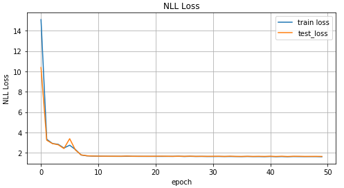
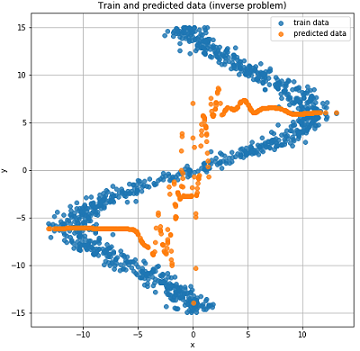
Graph of values of loss function depending on the iteration of training, on the graph of values for training data and test data.
Since our network has learned the mean values for several distributions, let's look at it:
pi, mu, sigma_sq = mdn_net(Variable(torch.from_numpy(x_test_inv)))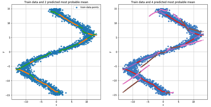
The graph for the two most likely mean values for each point (left). The graph for the 4 most likely mean values for each point (right).
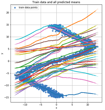
Graph for all mean values for each point.
To predict the data, we will randomly choose several values.
and based on the value . And then based on them generate target data using normal distribution.Result prediction
defrand_n_sample_cumulative(pi, mu, sigmasq, samples=10):
    n = pi.shape[0]
    out = Variable(torch.zeros(n, samples, OUT_DIM))
    for i in range(n):
        for j in range(samples):
            u = np.random.uniform()
            prob_sum = 0for k in range(COEFS):
                prob_sum += pi.data[i, k]
                if u < prob_sum:
                    for od in range(OUT_DIM):
                        sample = np.random.normal(mu.data[i, k*OUT_DIM+od], np.sqrt(sigmasq.data[i, k]))
                        out[i, j, od] = sample
                    breakreturn out
pi, mu, sigma_sq = mdn_net(Variable(torch.from_numpy(x_test_inv)))
preds = rand_n_sample_cumulative(pi, mu, sigma_sq, samples=10)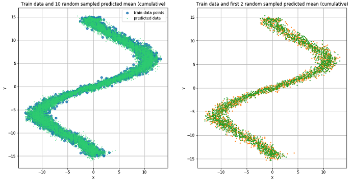
Predicted data for 10 randomly selected values.
and (left) and two (right). The figures show that MDN did an excellent job with the “reverse” task.
Using more complex data
Let's see how our MD network will cope with more complex data, such as spiral data. The equation of a hyperbolic spiral in Cartesian coordinates:

Spiral Data Generation
N = 2000
x_train_compl = []
y_train_compl = []
x_test_compl = []
y_test_compl = []
noise_train = np.random.uniform(-1, 1, (N, IN_DIM)).astype(np.float32)
noise_test = np.random.uniform(-1, 1, (N, IN_DIM)).astype(np.float32)
for i, theta in enumerate(np.linspace(0, 5*np.pi, N).astype(np.float32)):
    # формула 6
    r = ((theta))
    x_train_compl.append(r*np.cos(theta) + noise_train[i])
    y_train_compl.append(r*np.sin(theta))
    x_test_compl.append(r*np.cos(theta) + noise_test[i])
    y_test_compl.append(r*np.sin(theta))
x_train_compl = np.array(x_train_compl).reshape((-1, 1))
y_train_compl = np.array(y_train_compl).reshape((-1, 1))
x_test_compl = np.array(x_test_compl).reshape((-1, 1))
y_test_compl = np.array(y_test_compl).reshape((-1, 1))
Graph of the obtained spiral data.
For the sake of interest, let's see how the usual Feed-Forward network will cope with this task.
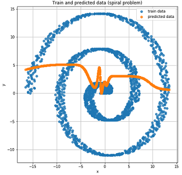
As expected, the Feed-Forward network is not able to solve the regression problem for such data.
We use the previously described and created MD network for training on spiral data.
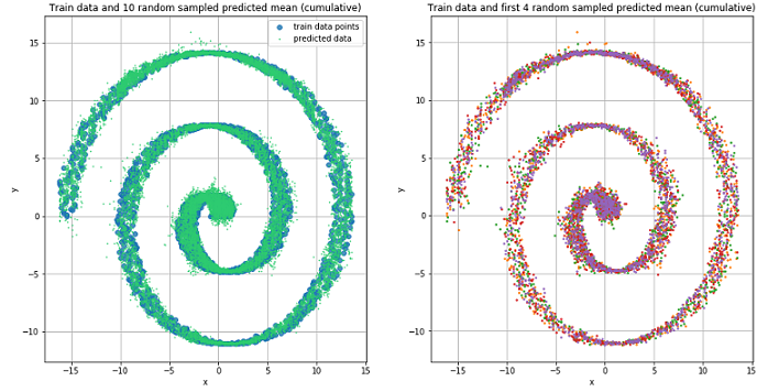
Mixture Density Network did a great job in this situation.
Conclusion
At the beginning of this article, we recalled the basics of linear regression. Saw that the general between finding of an average for normal distribution and MSE. Disassembled as related NLL and cross entropy. And most importantly, we figured out the MDN model, which is capable of learning from data obtained from a mixed distribution. I hope the article was clear and interesting, despite the fact that there was a bit of mathematics.
The full code can be viewed on GitHub .