Random forest vs neural networks: who will better cope with the task of recognizing sex in speech (Part 2)
The first part of our guide was devoted to an interesting task of machine learning - gender recognition by voice. We described a general approach to most speech processing tasks and, using a random forest trained on the statistics of acoustic features, we solved the problem with fairly high accuracy - 98.4% of correctly classified audio fragments.
In the second part of the guide, we will see whether neural networks can cope with this task more effectively than a random forest, and also try to take into account the biggest drawback of classical methods - the inability to work with data sequences.
In a sense, this step is redundant: the person’s gender does not change during the conversation (at least at the current stage of development and in the given standard conditions), so you should not count on an increase in accuracy. But for academic purposes, we will try. / Photo Tristan Bowersox / CC-SA

It is believed that an artificial neural network (neural network) is a mathematical model of the human brain. Actually not : 50-60 years ago, biologists at a certain level studied electrical processes in the brain, and mathematicians created a simplified model and programmed it.
It turned out that such structures are capable of solving some simple problems, but a) are worse than classical methods and b) are much slower than them. And the undeniable status quo was maintained for half a century - scientists developed the theory (teaching methods, architectures, fundamental mathematical questions), and computer technology and software developed so much that it became possible to solve some problems on a home PC at a global level.
But not allso smoothly: a neural network can learn to distinguish a cheetah from a leopard, or it can count a spotted sofa as one of these animals. In addition, the processes of teaching a person and a machine are different: a computer needs thousands of training examples, while a few are enough for a person. Obviously, the work of artificial neural networks is not very similar to human thinking, and they are not a computer model of the brain, but just another class of models on the list: Random Forest, SVM, XGBoost, etc., albeit with advantageous features.
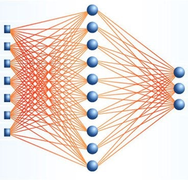
Historically, the first working architecture of a neural network is a multilayer perceptron. It consists of layers, and each layer is made up of neurons. The signal is transmitted in one direction - from the first layer to the last, and each neuron of the current layer is connected to all neurons of the previous one, and with different weights. The weight of the connection between two neurons has the physical meaning of its significance: the greater its value, the greater the contribution will be made to the output value of the neuron. To train a neural network is to find such values of weights that on the output layer we get what we need.
Fully connected architectures do not qualitatively differ from classical methods: they take a vector of numbers as an input, process them somehow, and the result is a set of probabilities of the input vector belonging to one of the classes (this is so for the classification problem, but others can be considered). In practice, other architectures (convolutional, recurrent) are used to process input features, receiving the so-called high-level features, and then they are processed using fully connected layers.
Analysis of the work of convolution networks can be found here and here.(there are thousands of them, so we leave the choice to the reader), and we will analyze recurrent ones separately. They take sequences of numbers as input, no matter whether it is signs, signal values, or word labels. The role of neurons for them is usually performed by special cells, which, in addition to summing the input signal and obtaining the output, have a set of additional parameters - internal values that are remembered and affect the output value of the cell.
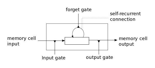
Today, the most widely used recurrent architecture is Long Short-Term Memory (LSTM). In the simplest implementation, in each cell, there are three special elements: input, output, and forget valve. They determine in what proportions it is necessary to “mix” the processed input data and the stored values so that the most useful signal is output. To train an LSTM network is to find such parameters of gates and the weights of connections between LSTM cells on the first layers and neurons of the last layers, for which for the input sequence the output layer would return the probability of belonging to each of the classes.
We hope you read the first part of this guide. In it you can find a description of the speech base, the calculated features, as well as the results of the Random Forest classifier. He was trained on the statistics of attributes, calculated on good (up to a certain limit), filtered sections of speech - frames. For each sign, the mean, median, minimum and maximum values, as well as standard deviation, were considered.
Neural networks are more demanding on the number of training examples. In the last part, we studied on 436 audio fragments from 109 speakers (four statements for each), taken from the VCTK database. It turned out that not one of the neural network architectures we tested was able to learn to reasonable accuracy values, and we took more fragments - only 5000. However, the increased sample did not lead to a significant increase in accuracy - 98.5% of correctly classified fragments. The first experiment we want to do is to train a fully connected neural network on the same set of features.
We continue to write all the code in Python, we take the implementation of neural networks from Keras - the most convenient library through which you can implement the necessary architectures in a couple of lines.
We import everything we need:
We take the implementation of a random forest from sklearn, and from there - cross-validation by groups. From Keras we take the base class for models, layers, the Bidirectional wrapper, which allows the use of bidirectional LSTM, as well as the to_categorical function, which encodes class labels in one-hot vectors.
We read all the data:
And we get a sample:
Here we applied frequency filtering - we threw out from the consideration those sections of speech on which the pitch frequency was not determined. This can happen in two cases: the frame does not correspond to speech at all, or corresponds to consonants or whispers. In our task, we can throw out absolutely all frames without a pitch, but in many others, filtering should be done less greedily.
Next, you need to implement a fully connected neural network:
The first layer of the network is Batch Normalization . It eliminates the need to normalize data, and also speeds up the learning process and makes it possible to some extent to avoid retraining. First, each batch (a portion of data at each iteration of training) is normalized to its own mean and standard deviation, and then it is scaled using a linear transformation, the parameters of which are subject to optimization.
For about the same purpose, after each fully connected layer there are Dropoutlayers. They randomly select some of the neurons (in our case, half) of the previous layer and zero out their output values. This allows us to make the network more stable: even if we remove some of the links, it will still give the correct answer. Exactly for this reason, in practice, layers with twice the number of neurons and 50% dropout are more effective than conventional layers.
Dense - directly fully connected layers. Their outputs are a classical sum of input signals weighted with some weights, non-linearly converted using the activation function. On the first layers it is tanh , and on the last - softmaxso that the sum of the output signal is equal to one and corresponds to the probabilities of being in one of the classes. Model checkpoint is more of a decorative thing, rewriting the model after each era of training, only if the measure of error on the test sample - validation loss - is less than that of the previous saved model. This ensures that the most efficient model is written to model.weights .
It remains to describe the cross-validation process for speakers and compare the fully-connected network and random forest described above on the same data:
We obtained approximately the same accuracy values - 98.6% for a random forest and 98.7% for a neural network. You can probably optimize the parameters and get higher accuracy, but right away we’ll start with what it was all about: recurrent networks.
First you need to make a selection of sequences. Keras, despite its simplicity, is sometimes finicky, and here it is necessary that the input variables in the .fit or .fit_on_batch methods can be naturally converted to tensors. For example, sequences of different lengths (and this is exactly the case with us) do not possess this property.
This purely technical limitation of the library can be circumvented in several ways. The first is training on size 1 batches. The obvious disadvantages of this approach are the inapplicability of batch normalization and a catastrophic increase in training time.
The second way is to add zeros to the sequence (padding) to get the desired dimension. At first glance, this seems wrong, but the network is learning not to respond to such values. Also, these methods can be combined - split the length sequences into several groups, inside each hold padding and train.
We will consider sequences of length 100 - this corresponds to one second of speech. To do this, we trim the long sequences so that exactly 100 points remain, moreover, symmetrical about the middle, and supplement the short ones with zeros at the beginning and end to the desired length.
Bidirectional wrapper uses merge_mode to glue the outputs of the argument layer for a regular input sequence and in reverse order. In our case, this is an LSTM layer with 100 cells. The return_sequences flag determines whether the sequence of internal states of cells will be returned or only the last one will be returned.
Inside LSTM and after the recurrence layers, a dropout is applied , and after the last layer (for which return_sequences = False ) there is a softmax activation function. The model also compiles with the Rmsprop optimizer .- modification of stochastic gradient descent. In practice, it often turns out that it works better for recurrent networks, although this is not strictly proven and can always be different.
Hurrah! 99.1% correctly classified points on 5-fold cross-validation by speakers. This is the best result among all considered architectures.
The lion's share of machine learning guides, articles, and non-fiction materials are dedicated to image recognition. Very rarely - reinforcement training. Even less commonly is audio processing. Partly, probably, this is due to the fact that the methods “out of the box” for audio processing do not work, and you have to spend your time understanding processes, data preprocessing and other inevitable iterations. But it is complexity that makes the task interesting.
Recognizing sex seems a simple task, because a person copes with it almost accurately. But its solution by the methods of machine learning “head-on” demonstrates an accuracy of about 70%, which is objectively small. However, even simple algorithms can achieve an accuracy of about 97-98% if everything is done correctly: for example, filter out the source data. Sophisticated neural network approaches increase accuracy to more than 99%, which is hardly fundamentally different from human performance.
In fact, the potential of recurrent neural networks in this article is not fully disclosed. Even for the classification task (many to one), they can be used more efficiently. But, of course, we will not do this yet. We offer readers to do without filtering frames, allowing the network itself to learn how to process only the necessary frames, and consider longer (or shorter, or thinned) sequences.
Worked on the material:
Stay with us.
In the second part of the guide, we will see whether neural networks can cope with this task more effectively than a random forest, and also try to take into account the biggest drawback of classical methods - the inability to work with data sequences.
In a sense, this step is redundant: the person’s gender does not change during the conversation (at least at the current stage of development and in the given standard conditions), so you should not count on an increase in accuracy. But for academic purposes, we will try. / Photo Tristan Bowersox / CC-SA
The next chapter on how neural networks work
It is believed that an artificial neural network (neural network) is a mathematical model of the human brain. Actually not : 50-60 years ago, biologists at a certain level studied electrical processes in the brain, and mathematicians created a simplified model and programmed it.
It turned out that such structures are capable of solving some simple problems, but a) are worse than classical methods and b) are much slower than them. And the undeniable status quo was maintained for half a century - scientists developed the theory (teaching methods, architectures, fundamental mathematical questions), and computer technology and software developed so much that it became possible to solve some problems on a home PC at a global level.
But not allso smoothly: a neural network can learn to distinguish a cheetah from a leopard, or it can count a spotted sofa as one of these animals. In addition, the processes of teaching a person and a machine are different: a computer needs thousands of training examples, while a few are enough for a person. Obviously, the work of artificial neural networks is not very similar to human thinking, and they are not a computer model of the brain, but just another class of models on the list: Random Forest, SVM, XGBoost, etc., albeit with advantageous features.
Historically, the first working architecture of a neural network is a multilayer perceptron. It consists of layers, and each layer is made up of neurons. The signal is transmitted in one direction - from the first layer to the last, and each neuron of the current layer is connected to all neurons of the previous one, and with different weights. The weight of the connection between two neurons has the physical meaning of its significance: the greater its value, the greater the contribution will be made to the output value of the neuron. To train a neural network is to find such values of weights that on the output layer we get what we need.
Fully connected architectures do not qualitatively differ from classical methods: they take a vector of numbers as an input, process them somehow, and the result is a set of probabilities of the input vector belonging to one of the classes (this is so for the classification problem, but others can be considered). In practice, other architectures (convolutional, recurrent) are used to process input features, receiving the so-called high-level features, and then they are processed using fully connected layers.
Analysis of the work of convolution networks can be found here and here.(there are thousands of them, so we leave the choice to the reader), and we will analyze recurrent ones separately. They take sequences of numbers as input, no matter whether it is signs, signal values, or word labels. The role of neurons for them is usually performed by special cells, which, in addition to summing the input signal and obtaining the output, have a set of additional parameters - internal values that are remembered and affect the output value of the cell.
Today, the most widely used recurrent architecture is Long Short-Term Memory (LSTM). In the simplest implementation, in each cell, there are three special elements: input, output, and forget valve. They determine in what proportions it is necessary to “mix” the processed input data and the stored values so that the most useful signal is output. To train an LSTM network is to find such parameters of gates and the weights of connections between LSTM cells on the first layers and neurons of the last layers, for which for the input sequence the output layer would return the probability of belonging to each of the classes.
Initial settings
We hope you read the first part of this guide. In it you can find a description of the speech base, the calculated features, as well as the results of the Random Forest classifier. He was trained on the statistics of attributes, calculated on good (up to a certain limit), filtered sections of speech - frames. For each sign, the mean, median, minimum and maximum values, as well as standard deviation, were considered.
Neural networks are more demanding on the number of training examples. In the last part, we studied on 436 audio fragments from 109 speakers (four statements for each), taken from the VCTK database. It turned out that not one of the neural network architectures we tested was able to learn to reasonable accuracy values, and we took more fragments - only 5000. However, the increased sample did not lead to a significant increase in accuracy - 98.5% of correctly classified fragments. The first experiment we want to do is to train a fully connected neural network on the same set of features.
We continue to write all the code in Python, we take the implementation of neural networks from Keras - the most convenient library through which you can implement the necessary architectures in a couple of lines.
We import everything we need:
import csv, os
import numpy as np
import sklearn
from sklearn.ensemble import RandomForestClassifier as RFC
from sklearn.model_selection import GroupKFold
from keras.models import Model
from keras.callbacks import ModelCheckpoint
from keras.layers import Input, Dense, Dropout, LSTM, Activation, BatchNormalization
from keras.layers.wrappers import Bidirectional
from keras.utils import to_categorical
We take the implementation of a random forest from sklearn, and from there - cross-validation by groups. From Keras we take the base class for models, layers, the Bidirectional wrapper, which allows the use of bidirectional LSTM, as well as the to_categorical function, which encodes class labels in one-hot vectors.
We read all the data:
with open('data.csv', 'r')as c:
	r = csv.reader(c, delimiter=',')
	header = next(r)
	data = []
	for row in r:
		data.append(row)
data = np.array(data)
genders = data[:, 0].astype(int)
speakers = data[:, 1].astype(int)
filenames = data[:, 2]
times = data[:, 3].astype(float)
pitch = data[:, 4:5].astype(float)
features = data[:, 4:].astype(float)
And we get a sample:
def make_sample(x, y, subj, names, statistics=[np.mean, np.std, np.median, np.min, np.max]):
	avx = []
	avy = []
	avs = []
	keys = np.unique(names)
	for ki, k in enumerate(keys):
		idx = names == k
		v = []
		for stat in statistics:
			v += stat(x[idx], axis=0).tolist()
		avx.append(v)
		avy.append(y[idx][0])
		avs.append(subj[idx][0])
	return np.array(avx), np.array(avy).astype(int), np.array(avs).astype(int)
filter_idx = pitch[:, 0] > 1
filtered_average_features, filtered_average_genders, filtered_average_speakers = make_sample(features[filter_idx], genders[filter_idx], speakers[filter_idx], filenames[filter_idx])
Here we applied frequency filtering - we threw out from the consideration those sections of speech on which the pitch frequency was not determined. This can happen in two cases: the frame does not correspond to speech at all, or corresponds to consonants or whispers. In our task, we can throw out absolutely all frames without a pitch, but in many others, filtering should be done less greedily.
Next, you need to implement a fully connected neural network:
def train_dnn(x, y, tx, ty):
	yc = to_categorical(y) # one-hot encoding for y
	tyc = to_categorical(ty)# one-hot encoding for y_test
	inp = Input(shape=(x.shape[1],))
	model = BatchNormalization()(inp)
	model = Dense(100, activation='tanh')(model)
	model = Dropout(0.5)(model)
	model = Dense(100, activation='tanh')(model)
	model = Dropout(0.5)(model)
	model = Dense(100, activation='sigmoid')(model)
	model = Dense(2, activation='softmax')(model)
	model = Model(inputs=[inp], outputs=[model])
	model.compile(optimizer='sgd', loss='categorical_crossentropy', metrics=['acc'])
	modelcheckpoint = ModelCheckpoint('model.weights', monitor='val_loss', verbose=1, save_best_only=True, mode='min')
	model.fit(x, yc, validation_data=(tx, tyc), epochs=100, batch_size=100, callbacks=[modelcheckpoint], verbose=2)
	model.load_weights('model.weights')
	return model
The first layer of the network is Batch Normalization . It eliminates the need to normalize data, and also speeds up the learning process and makes it possible to some extent to avoid retraining. First, each batch (a portion of data at each iteration of training) is normalized to its own mean and standard deviation, and then it is scaled using a linear transformation, the parameters of which are subject to optimization.
For about the same purpose, after each fully connected layer there are Dropoutlayers. They randomly select some of the neurons (in our case, half) of the previous layer and zero out their output values. This allows us to make the network more stable: even if we remove some of the links, it will still give the correct answer. Exactly for this reason, in practice, layers with twice the number of neurons and 50% dropout are more effective than conventional layers.
Dense - directly fully connected layers. Their outputs are a classical sum of input signals weighted with some weights, non-linearly converted using the activation function. On the first layers it is tanh , and on the last - softmaxso that the sum of the output signal is equal to one and corresponds to the probabilities of being in one of the classes. Model checkpoint is more of a decorative thing, rewriting the model after each era of training, only if the measure of error on the test sample - validation loss - is less than that of the previous saved model. This ensures that the most efficient model is written to model.weights .
It remains to describe the cross-validation process for speakers and compare the fully-connected network and random forest described above on the same data:
def subject_cross_validation(clf, x, y, subj, folds):
	gkf = GroupKFold(n_splits=folds)
	scores = []
	for train, test in gkf.split(x, y, groups=subj):
		if clf == 'dnn':
			model = train_dnn(x[train], y[train], x[test], y[test])
			score = model.evaluate(x[test], to_categorical(y[test]))[1]
			scores.append(score)
		elif clf == 'lstm':
			model = train_lstm(x[train], y[train], x[test], y[test])
			score = model.evaluate(x[test], to_categorical(y[test]))[1]
			scores.append(score)
		else:
			clf.fit(x[train], y[train])
			scores.append(clf.score(x[test], y[test]))
	return np.mean(scores)
score_filtered = subject_cross_validation(RFC(n_estimators=1000), filtered_average_features, filtered_average_genders, filtered_average_speakers, 5)
print score_filtered
score_filtered = subject_cross_validation('dnn', filtered_average_features, filtered_average_genders, filtered_average_speakers, 5)
print('Utterance classification an averaged features over filtered frames, accuracy:', score_filtered)
We obtained approximately the same accuracy values - 98.6% for a random forest and 98.7% for a neural network. You can probably optimize the parameters and get higher accuracy, but right away we’ll start with what it was all about: recurrent networks.
def make_sequences(x, y, subj, names):
	sx = []
	sy = []
	ss = []
	keys = np.unique(names)
	sequence_length = 100
	for ki, k in enumerate(keys):
		idx = names == k
		v = x[idx]
		w = np.zeros((sequence_length, v.shape[1]), dtype=float)
		sh = v.shape[0]
		if sh <= sequence_length:
			dh = sequence_length - sh
			if dh % 2 == 0:
				w[dh//2:sequence_length-dh//2, :] = v
			else:
				w[dh//2:sequence_length-1-dh//2, :] = v
		else:
			dh = sh - sequence_length
			w = v[sh//2-sequence_length//2:sh//2+sequence_length//2, :]
		sx.append(w)
		sy.append(y[idx][0])
		ss.append(subj[idx][0])
	return np.array(sx), np.array(sy).astype(int), np.array(ss).astype(int)
First you need to make a selection of sequences. Keras, despite its simplicity, is sometimes finicky, and here it is necessary that the input variables in the .fit or .fit_on_batch methods can be naturally converted to tensors. For example, sequences of different lengths (and this is exactly the case with us) do not possess this property.
This purely technical limitation of the library can be circumvented in several ways. The first is training on size 1 batches. The obvious disadvantages of this approach are the inapplicability of batch normalization and a catastrophic increase in training time.
The second way is to add zeros to the sequence (padding) to get the desired dimension. At first glance, this seems wrong, but the network is learning not to respond to such values. Also, these methods can be combined - split the length sequences into several groups, inside each hold padding and train.
We will consider sequences of length 100 - this corresponds to one second of speech. To do this, we trim the long sequences so that exactly 100 points remain, moreover, symmetrical about the middle, and supplement the short ones with zeros at the beginning and end to the desired length.
def train_lstm(x, y, tx, ty):
	yc = to_categorical(y)
	tyc = to_categorical(ty)
	inp = Input(shape=(x.shape[1], x.shape[2]))
	model = BatchNormalization()(inp)
	model = Bidirectional(LSTM(100, return_sequences=True, recurrent_dropout=0.1), merge_mode='concat')(model)
	model = Dropout(0.5)(model)
	model = Bidirectional(LSTM(100, return_sequences=True, recurrent_dropout=0.1), merge_mode='concat')(model)
	model = Dropout(0.5)(model)
	model = Bidirectional(LSTM(2, return_sequences=False, recurrent_dropout=0.1), merge_mode='ave')(model)
	model = Activation('softmax')(model)
	model = Model(inputs=[inp], outputs=[model])
	model.compile(optimizer='rmsprop', loss='categorical_crossentropy', metrics=['acc'])
	modelcheckpoint = ModelCheckpoint('model.weights', monitor='val_loss', verbose=1, save_best_only=True, mode='min')
	model.fit(x, yc, validation_data=(tx, tyc), epochs=100, batch_size=50, callbacks=[modelcheckpoint], verbose=2)
	model.load_weights('model.weights')
	return model
Bidirectional wrapper uses merge_mode to glue the outputs of the argument layer for a regular input sequence and in reverse order. In our case, this is an LSTM layer with 100 cells. The return_sequences flag determines whether the sequence of internal states of cells will be returned or only the last one will be returned.
Inside LSTM and after the recurrence layers, a dropout is applied , and after the last layer (for which return_sequences = False ) there is a softmax activation function. The model also compiles with the Rmsprop optimizer .- modification of stochastic gradient descent. In practice, it often turns out that it works better for recurrent networks, although this is not strictly proven and can always be different.
filter_idx = pitch[:, 0] > 1
filtered_sequences_features, filtered_sequences_genders, filtered_sequences_speakers = make_sequences(features[filter_idx], genders[filter_idx], speakers[filter_idx], filenames[filter_idx])
score_lstmfiltered = subject_cross_validation('lstm', filtered_sequences_features, filtered_sequences_genders, filtered_sequences_speakers, 5)
print score_lstm_filtered
Hurrah! 99.1% correctly classified points on 5-fold cross-validation by speakers. This is the best result among all considered architectures.
Conclusion
The lion's share of machine learning guides, articles, and non-fiction materials are dedicated to image recognition. Very rarely - reinforcement training. Even less commonly is audio processing. Partly, probably, this is due to the fact that the methods “out of the box” for audio processing do not work, and you have to spend your time understanding processes, data preprocessing and other inevitable iterations. But it is complexity that makes the task interesting.
Recognizing sex seems a simple task, because a person copes with it almost accurately. But its solution by the methods of machine learning “head-on” demonstrates an accuracy of about 70%, which is objectively small. However, even simple algorithms can achieve an accuracy of about 97-98% if everything is done correctly: for example, filter out the source data. Sophisticated neural network approaches increase accuracy to more than 99%, which is hardly fundamentally different from human performance.
In fact, the potential of recurrent neural networks in this article is not fully disclosed. Even for the classification task (many to one), they can be used more efficiently. But, of course, we will not do this yet. We offer readers to do without filtering frames, allowing the network itself to learn how to process only the necessary frames, and consider longer (or shorter, or thinned) sequences.
Worked on the material:
- Grigory Sterling , mathematician, leading Neurodata Lab expert on machine learning and data analysis
- Eva Kazimirova , biologist, physiologist, Neurodata Lab expert in the field of acoustics, analysis of voice and speech signals
Stay with us.