Deep Learning Research Survey: Natural Language Processing

This is the third article in the series “Deep Learning Research Review” by Adit Deshpande, a student at the University of California, Los Angeles. Every two weeks, Adit publishes a review and interpretation of research in a specific area of ​​deep learning. This time he focused on the use of deep learning to process natural language texts.

Introduction to Natural Language Processing

Introduction

Natural Language Processing (NLP) refers to the creation of systems that process or “understand” a language in order to perform certain tasks. These tasks may include:

• Forming answers to questions (Question Answering) (what Siri, Alexa and Cortana do)
• Sentiment Analysis (determining whether a statement has a positive or negative connotation)
• Finding text that matches the image (Image to Text Mappings) (generating a caption for the input image)
• Machine Translation (Translation of a paragraph of text from one language to another)
• Speech Recognition
• Morphological markup (Part of Speech Tagging) (definition of parts of speech in a sentence and their annotation)
• Entity Recognition

The traditional approach to NLP assumed a deep knowledge of the subject area - linguistics. An understanding of terms such as phonemes and morphemes was mandatory, as there are entire disciplines of linguistics dedicated to their study. Let's see how the traditional NLP would recognize the following word:

Suppose our goal is to collect some information about this word (determine its emotional coloring, find its meaning, etc.). Using our knowledge of the language, we can break this word into three parts.


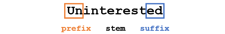
We understand that the prefix un- means negation, and we know that -ed can mean the time to which a given word refers (in this case, past tense). Having recognized the meaning of the root word interest, we can easily conclude the meaning and emotional coloring of the whole word. It seems to be simple. Nevertheless, if you take into account the whole variety of prefixes and suffixes of the English language, you will need a very skilled linguist to understand all the possible combinations and their meanings.


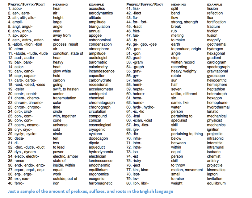
An example showing the number of prefixes of suffixes and roots in English

How to use deep learning

At the heart of deep learning is learning to represent. For example, convolutional neural networks (CNN) include a combination of various filters designed to classify objects into categories. Here we will try to apply a similar approach, creating representations of words in large data sets.

Article structure

This article is organized in such a way that we can go through the basic elements from which you can build deep networks for NLP, and then proceed to discuss some of the applications that concern recent scientific work. It’s okay if you don’t know exactly why, for example, we use RNN, or what LSTM is useful for, but hopefully after studying these works, you will understand why deep learning is so important for NLP.

Words vectors

Since deep learning cannot live without mathematics, we represent each word as a d-dimensional vector. Take d = 6.

Now consider how to fill in the values. We want the vector to be filled in such a way that it somehow represents the word and its context, meaning or semantics. One way is to build a cooccurrence matrix. Consider the following sentence:

We want a vector representation for each word.


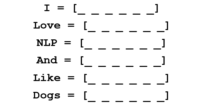
The co-occurrence matrix contains the number of times that each word occurs in the corpus (training set) after each other word of this corpus.



The rows of this matrix can serve as vector representations of our words.

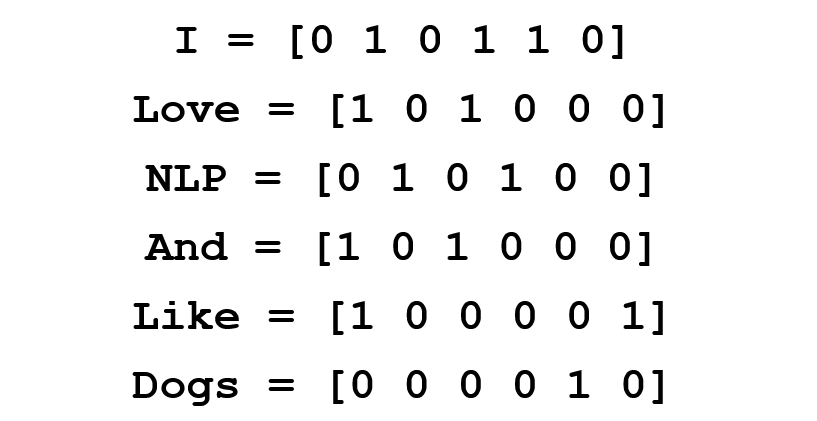
Please note that even from this simple matrix, we can draw some pretty important information. For example, note that the vectors of the words “love” and “like” contain units in the cells that are responsible for their proximity to nouns (“NLP” and “dogs”). They also have “1” where they are adjacent to “I”, indicating that this word is most likely a verb. You can imagine how much easier it is to identify similar similarities when the data set is more than one sentence: in this case, the vectors of such verbs like “love”, “like” and other synonyms will be similar, since these words will be used in similar contexts.

Good for a start, but here we pay attention that the dimension of the vector of each word will increase linearly depending on the size of the corpus. In the case of a million words (which is not enough for standard NLP tasks), we would get a matrix of dimension one million per million, which, moreover, would be very sparse (with a large number of zeros). This is definitely not the best option in terms of storage efficiency. In the matter of finding the optimal vector representation of words, several serious advances have been made. The most famous of them is Word2Vec.

Word2vec

The main goal of all methods of initializing a word vector is to store as much information as possible in this vector, while maintaining a reasonable dimension (ideally, from 25 to 1000). At the core of Word2Vec is the idea of ​​learning how to predict the surrounding words for each word. Consider the sentence from the previous example: “I love NLP and I like dogs”. Now we are only interested in the first three words. Let the size of our window be three.

Now we want to take the central word “love” and predict the words that come before and after it. How do we do this? Of course, by maximizing and optimizing the function! Formally, our function tries to maximize the logarithmic probability of each context word for the current central word.

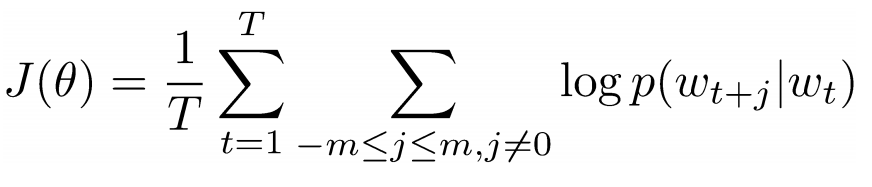
We study the above formula in more detail. It follows from it that we will add up the logarithmic probability of joint occurrence of both “I” and “love”, and “NLP” and “love” (in both cases “love” is the central word). The variable T means the number of training proposals. Consider the logarithmic probability closer.

$$- vector representation of the central word. Each word has two vector representations:$$ and $$, one for the case when the word occupies a central position, the other for the case when this word is “external”. Vectors are trained by stochastic gradient descent. This is definitely one of the most difficult equations to understand, so if you’re still having a hard time imagining what’s going on, you can find more information here and here .

To summarize in one sentence : Word2Vec searches for vector representations of various words, maximizing the logarithmic probability of occurrence of context words for a given central word and transforming the vectors by stochastic gradient descent.

(Optional: on the authors of the workdescribe in detail how using negative sampling and subsampling you can get more accurate word vectors).

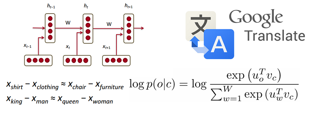
Perhaps the most interesting contribution of Word2Vec to the development of NLP was the emergence of linear relationships between different word vectors. After training, vectors reflect various grammatical and semantic concepts.

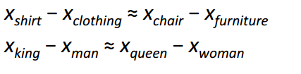
It is amazing how such a simple objective function and a simple optimization technique were able to identify these linear relationships.

Bonus : Another cool method for initializing word vectors is GloVe (Global Vector for Word Representation) (combines the ideas of a co-occurrence matrix with Word2Vec).

Recurrent Neural Networks (RNN)

Now let's see how a recurrent neural network will work with our vectors. RNN is a lifesaver for most modern natural language processing tasks. The main advantage of RNNs is that they can efficiently use the data from the previous steps. This is what a small piece of RNN looks like:

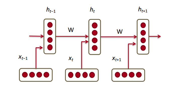
At the bottom are the word vectors ($$) Each vector at each step has a hidden state vector (hidden state vector) ($$) We will call this pair a module.

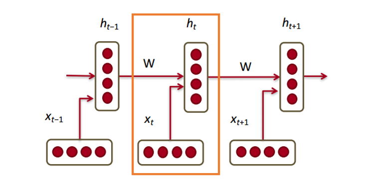
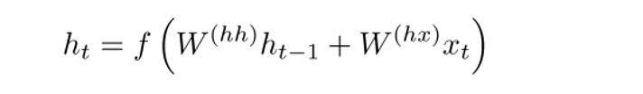
The latent state in each RNN module is a function of the word vector and the latent state vector from the last step.

If we look closely at the superscripts, we will see that there is a weight matrix$$, which we multiply by the input value, is the recurrence matrix of weights $$, which is multiplied by the hidden state vector from the previous step. Keep in mind that these recurrence weight matrices are the same at every step. This is the key point of RNN . If you think carefully, this approach is significantly different from, say, traditional two-layer neural networks. In this case, we usually select a separate matrix W for each layer:$$ and $$. Here, the recurrence matrix of weights is the same for the entire network.

To obtain the output values ​​of each module (Yhat) is another matrix of weights -$$times h.


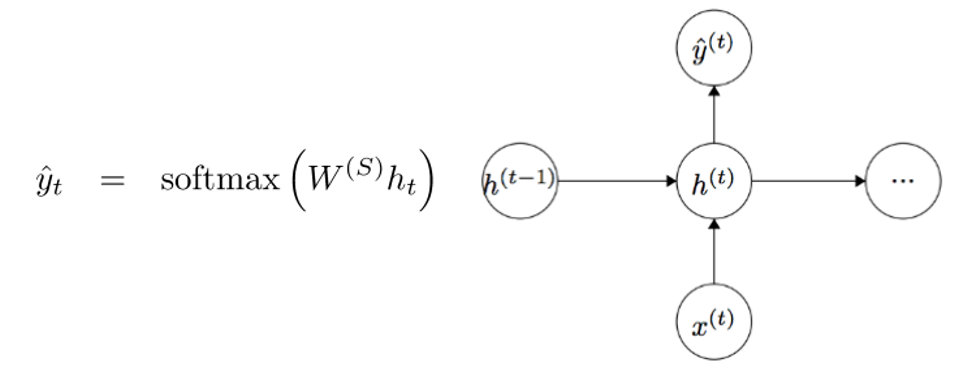
Now let's look from the outside and understand what the advantages of RNN are. The most obvious difference between RNN and traditional neural network is that RNN receives a sequence of input data (in our case, words) as input. In this they differ, for example, from typical CNNs, to the input of which a whole image is supplied. For RNN, however, both a short sentence and an essay of five paragraphs can serve as input. In addition, the order in which data is presented can affect how the weight matrices and vectors of latent states change during training. By the end of the training, the information from the previous steps should accumulate in the vectors of hidden states.

Controlled Recurrent Neurons (Gated recurrent units, GRU)

Now let's get acquainted with the concept of a controlled recurrent neuron, with the help of which the hidden state vectors are calculated in RNN. This approach allows you to save information about more distant dependencies. Let's talk about why long-distance dependencies for regular RNNs can be a problem. While the backpropagation method is running, the error will move along the RNN from the last step to the earliest. With a sufficiently small initial gradient (say, less than 0.25) for the third or fourth module, the gradient will almost disappear (since the gradients will multiply by the rule of the derivative of a complex function), and then the hidden states of the very first steps will not be updated.

In ordinary RNNs, the hidden state vector is calculated using the following formula:

The GRU method allows one to calculate h (t) differently. The calculations are divided into three blocks: an update gate filter, a reset gate filter, and a new memory container. Both filters are functions of the input vector representation of the word and the hidden state in the previous step.

The main difference is that each filter uses its own weight. This is indicated by different superscripts. Update filter uses$$ and $$and the status reset filter is $$ and $$.
Now let's calculate the memory container:

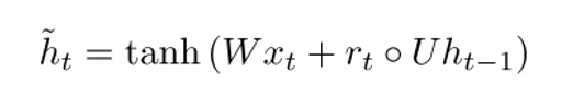
(an empty circle here indicates the product of Hadamard ).

Now, if you look closely at the formula, you can see that if the multiplier of the state reset filter is close to zero, then the whole product will also approach zero, and thus, the information from the previous step$$will not be counted. In this case, the neuron is just a function of the new word vector$$.

The final formula h (t) can be written as

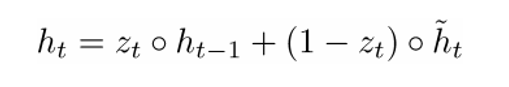
$$- a function of all three components: an update filter, a status reset filter, and a memory container. You can better understand this by visualizing what happens to the formula when$$ approaching 1 and when $$ close to 0. In the first case, the hidden state vector $$ to a greater extent depends on the previous hidden state, and the current memory container is not taken into account, since (1 - $$) tends to 0. But when $$ approaching 1, a new hidden state vector $$on the contrary, it depends mainly on the memory container, and the previous hidden state is not taken into account. So, our three components can be intuitively described as follows:

• Update filter
  
  • If $$ ~ 1 then $$ does not take into account the current word vector and simply copies the previous hidden state.
  • If $$ ~ 0 then $$ does not take into account the previous hidden state and depends only on the memory container.
  • This filter allows the model to control how much information from the previous hidden state should affect the current hidden state.
• Status Reset Filter
  
  • If $$ ~ 1, then the memory container stores information from the previous hidden state.
  • If $$ ~ 0, then the memory container does not take into account the previous hidden state.
  • This filter allows you to discard some of the information if in the future it will not interest us.
• Memory container: Depends on the status reset filter.

We give an example illustrating the operation of GRU. Suppose we have the following several sentences:

and the question: “What is the sum of two numbers?” Since the sentence in the middle does not affect the answer in any way, the reset and update filters will allow the model to “forget” this sentence and understand that only certain information (in this case, numbers) can change the hidden state.

Neurons with long short-term memory (LSTM)

If you figured out GRU, then LSTM will not be difficult for you. LSTM also consists of a sequence of filters.

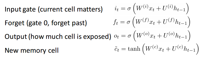
LSTM definitely accepts more input. Since it can be considered an extension of GRU, I will not analyze it in detail, and to get a detailed description of each filter and each step of the calculations, you can refer to the beautifully written blog post by Chris Olah. This is currently the most popular tutorial on LSTM, and will definitely help those of you who are looking for an understandable and intuitive explanation of how this method works.

Comparison of LSTM and GRU

First, consider the common features. Both of these methods are designed to preserve distant dependencies in word sequences. By distant dependencies we mean situations where two words or phrases can occur at different time steps, but the relationship between them is important to achieve the ultimate goal. LSTM and GRU track this relationship using filters that can save or discard information from the sequence being processed.

The difference between the two methods is the number of filters (GRU - 2, LSTM - 3). This affects the amount of non-linearity that comes from the input and ultimately affects the calculation process. In addition, there is no memory location in GRU.$$as in LSTM.

Before delving into the articles

I would like to make a small remark. If other deep learning models useful in NLP. In practice, recursive and convolutional neural networks are sometimes used, although they are not as common as the RNNs that underlie most NLP deep learning systems.

Now that we have begun to be well versed in recurrent neural networks in relation to NLP, let's take a look at some of the work in this area. Since NLP includes several different areas of tasks (from machine translation to generating answers to questions), we could consider quite a few works, but I chose the three that I found particularly informative. In 2016, there have been a number of major advancements in the field of NLP, but let's start with one work in 2015.

Neural networks with memory (Memory Networks)

Introduction

The first work that we will discuss has had a great influence on the development of the field of forming answers to questions. In this publication by Jason Weston, Sumit Chopra and Antoine Bordes, a class of models called “memory networks” was first described.

The intuitive idea is this: in order to accurately answer the question relating to the text fragment, it is necessary to somehow store the initial information provided to us. If I asked you: “What does the abbreviation RNN mean?”, You could answer me because the information that you learned while reading the first part of the article was stored somewhere in your memory. It would take you just a few seconds to find this information and voice it. I have no idea how this works in the brain, but the idea that space is needed to store this information remains unchanged.

The network with memory described in this paper is unique, since it has an associative memory to which it can write and from which it can read. It is interesting to note that neither CNN nor Q-Network (for reinforcement learning), nor traditional neural networks use this memory. This is partly due to the fact that the task of generating answers to questions relies heavily on the ability to simulate or to trace distant dependencies, for example, to follow the heroes of history or to remember the sequence of events.In CNN or Q-Networks, the memory is built into the weight of the system, as it learns various filters or maps of state and action correspondences. look, one could use RNN or LSTM,

Network architecture

Now let's see how such a network processes the source text. Like most machine learning algorithms, the first step is to transform the input into a representation in the attribute space. This may mean the use of vector representations of words, morphological markup, parsing, etc., at the discretion of the programmer.

The next step is to take a representation in the attribute space I (x) and read into the memory a new portion of the input data x.

Memory m can be regarded as a kind of array composed of separate memory blocks$$. Each such block$$can be a function of the entire memory m, the representation in space of signs I (x) and / or itself. The function G can simply store the entire representation of I (x) in the memory block mi. Function G can be changed so that it updates the memory of the past based on new input data. The third and fourth steps include reading from memory in the light of the question to find a representation of the characteristics of o, and decoding it to get the final answer r.

The function R can be RNN, which transforms the presentation of characters into human-readable and accurate answers to questions.

Now let's take a look at step 3. We want the O function to return the representation in the attribute space that best suits the possible answer to the given question x. We will compare this question with each individual memory block and evaluate how each block fits the answer to the question.

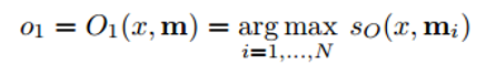
We find the maximization argument (argmax) of the evaluation function to find the representation that best matches the question (you can also select several blocks with the highest ratings, not necessarily exactly one). The evaluation function computes the matrix product between different vector representations of the question and the selected block (or blocks) of memory (for details, see the work itself). You can imagine this process as a multiplication of two two-word vectors to determine if they are equal. The output representation is then passed to RNN, LSTM, or another evaluation function that will return a human-readable answer.

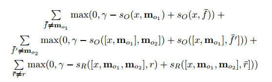
The network is trained using the teaching method with the teacher, when the training data includes the source text, the question, supporting sentences and the correct answer. Here's what the objective function looks like:



For those who are interested, here are a few more works based on the approach of memory networks:

• End to end memory networks
• Dynamic memory networks
• Dynamic Coattention Networks (implemented in November 2016 and got the best result of all time on the Stanford's Question Answering dataset)

Tree-LSTM for analysis of emotional coloring of statements

Introduction

The following work talks about progress in the field of analysis of emotional coloring - the task of determining whether it has a positive or negative connotation (meaning). Formally, emotional coloring can be defined as “a look at the situation or event or attitude towards them”. At that time, LSTM was the most common tool for recognizing emotional coloring. The work of authorship by Kai Sheng Tai, Richard Socher, and Christopher Manning introduces a fundamentally new way of combining several LSTM neurons into a nonlinear structure.

The idea of ​​a non-linear arrangement of components is based on the belief that natural languages ​​demonstrate the ability to turn sequences of words into phrases. These phrases, depending on the order of words, may have a meaning different from the initial value of the components included in them. To reflect this property, a network of several LSTM neurons should be presented in the form of a tree, where each child is affected by its child nodes.

Network architecture

One of the differences between Tree-LSTM and regular LSTM is that in the latter, the hidden state is a function of the current input and the hidden state in the previous step. In Tree-LSTM, the latent state is a function of the current input data and the hidden states of its child neurons.

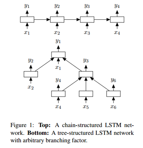
Along with the new structure - the tree - some changes are also introduced in the mathematics of the network, for example, daughter neurons now have forget filters. You can get acquainted with the details in the work itself. And I would like to pay attention to explaining why such networks work better than linear LSTMs.

In Tree-LSTM, each neuron can contain the hidden states of all its child nodes. This is an interesting point, since a neuron can evaluate each of its child nodes differently. During training, the network may realize that a certain word (for example, the word “not” or “very”) is extremely important for determining the emotional coloring of the whole sentence. The ability to rate the corresponding node higher provides greater network flexibility and can improve its performance.

Neural Machine Translation (NMT)

Introduction

The last work that we will consider today describes an approach to solving the problem of machine translation. The authors of this work - Google machine learning experts Jeff Dean, Greg Corrado, Orial Vinyals and others - represent the machine learning system that underlies the widely known Google Translate service. With the introduction of this system, the number of translation errors decreased by an average of 60% compared to the previous system used by Google.

Traditional approaches to automatic translation include finding phrase matches. This approach required a good knowledge of linguistics and in the end turned out to be insufficiently stable and incapable of generalization. One of the problems with the traditional approach was that the original sentence was translated piecemeal. It turned out that translating the whole sentence at a time (as NMT does) is more efficient, since in this case a wider context is involved and the word order becomes more natural.

Network architecture

The authors of this article describe the deep LSTM network, which can be trained using eight layer encoders and decoders. We can divide the system into three components: an RNN encoder, an RNN decoder, and an attention module. The encoder works on the task of converting the input sentence to a vector representation, the decoder returns the output representation, then the attention module tells the decoder what to focus on during the decoding operation (here comes the idea of ​​using the entire context of the sentence).

Further, the article focuses on the problems associated with the deployment and scaling of this service. It discusses topics such as computing resources, latency, and mass deployment of a service.

Conclusion

This concludes the post on how deep learning contributes to solving natural language processing problems. I think that further goals in the development of this area could be to improve chatbots for customer service, perfect machine translation and, possibly, training systems for answering questions deeply in unstructured or long texts (for example, Wikipedia pages).

Oh, and come to us to work? :)

wunderfund.io is a young foundation that deals with high-frequency algorithmic trading . High-frequency trading is a continuous competition of the best programmers and mathematicians around the world. By joining us, you will become part of this fascinating battle.

We offer interesting and complex data analysis and low latency development tasks for enthusiastic researchers and programmers. A flexible schedule and no bureaucracy, decisions are quickly taken and implemented.

Join our team: wunderfund.io