Preparing Physically Based Rendering + Image-based Lighting. Theory + practice. Step by step
 Hey hello. 2017 is in the yard. Even simple mobile and browser applications are slowly starting to draw physically correct lighting. The Internet is replete with a bunch of articles and ready-made shaders. And it seems like it should be so easy to smear PBR too ... Or not?
 In fact, honest PBR is difficult to do, because it is easy to achieve a similar result, but difficult to get it right. And the Internet is full of articles that do exactly the same result, instead of the correct one. Separating flies from cutlets in this chaos becomes difficult.
Therefore, the purpose of the article is not only to understand what PBR is and how it works, but also to learn how to write it. How to debug, where to look, and what mistakes can typically be made.
The article is intended for people who already know hlsl sufficiently and are familiar with linear algebra, and you can write your simplest non-PBR Phong light. In general, I will try to explain as simple as possible, but I hope that you already have some experience working with shaders.
The examples will be written in Delphi (and built under FreePascal), but the main code will still be in hlsl. Therefore, do not be scared if you do not know Delphi.
Where can I see and feel?
To build the examples, you need the AvalancheProject code . This is my framework around DX11 / OpenGL. Still need a Vampyre Imaging Library . This is a library for working with pictures, I use it to load textures. The source code for the examples is here . For those who do not want / cannot collect binaries, but want to use the already collected, they are here .
So fastened our seat belts, let's go.
1 Importance of sRGB Support
Our monitors usually display sRGB image. This is 95% true for desktops, and to some extent true for laptops (and on phones there is sheer arbitrariness).
This is due to the fact that our perception is not linear, and we notice better small changes in light in dark areas than the same absolute changes in bright areas. If it’s rough, then with a brightness increase of 4 times, we perceive this as a brightness increase of 2 times. I prepared a picture for you:

Before you try to understand the picture, make sure that your browser or operating system has not resized the image.
In the middle is a square consisting of horizontal single-pixel black and white stripes. The amount of light from this square is exactly 2 times less than from pure white. Now, if you move away from the screen so that the stripes merge into a square of the same color, then on a calibrated monitor, the central square should merge with the right square, and the left one will be much darker. If you now take the color of the left square with a pipette, you will find that it is 128, and the right square is 187. It turns out that when mixing 50/50 black: 0 0 0 and white 255 255 255 we get not ~ 128 128 128, but already 187 187 187.
Therefore, for a physically correct rendering, it is important for us that the white multiplied by 0.5 on the screen turns into 187 187 187. For this, the graphic APIs (DirectX and OpenGL) have hardware support for sRGB. At the moment of working with textures in the shader, they are transferred to linear space, and when displayed on the screen, they are transferred back to sRGB.
I will not dwell on how to achieve this in DirectX / OpenGL. It’s easy to google. And make sure that your sRGB earned quite simply. The linear gradient from black to white should change like this:
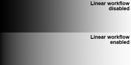
I just needed to show the importance of working in linear space, because this is one of the first mistakes that occurs on the Internet in articles about PBR.
2 Cook-Torrance
A physically correct render usually takes into account such things as:
- Fresnel reflection coefficients
- Law of energy conservation
- Theory micrograin ( microfacet theory ) for reflected light and re-emitted
The list can be expanded on microfacet theory for subsurface scattering and physically correct refraction, etc., but in the context of this article we will talk about the first three points.
2.1 Microfacet Theory
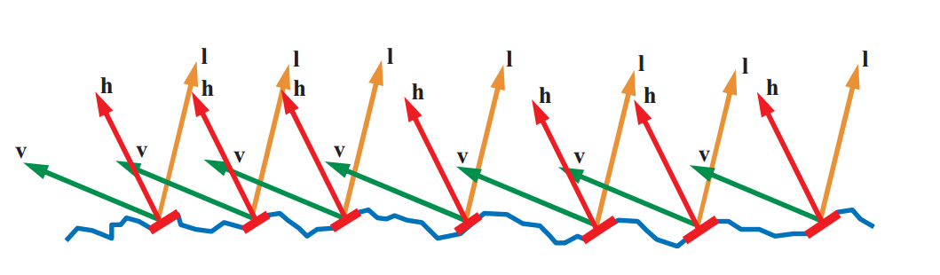
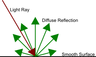
The surfaces of various materials in the real world are not absolutely smooth, but very rough. These irregularities are much longer than the light wavelength, and make a significant contribution to lighting. It is impossible to describe a rough plane with one normal vector, and the normal usually describes a certain average value of the macro-surface:
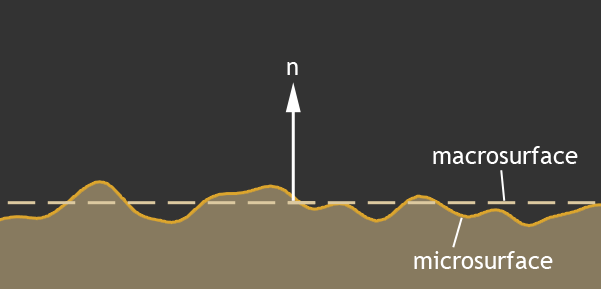
When in reality the micro-faces make the main contribution to the reflected light:
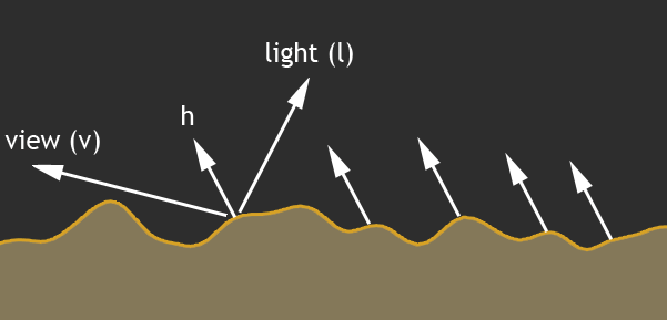
We all remember that the angle of incidence is equal to the angle of reflection, and the vector h in this figure describes exactly the normal micro-faces which contributes to lighting. It is the light from this point on the surface that we will see.
In addition, part of the world does not physically reach the micro-faces that could reflect it:
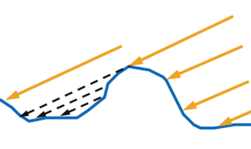
This is called self-shadowing, or self shadowing .
And the light that has flown to the surface and reflected will not always be able to fly out:
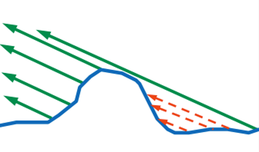
This is called self-overlapping, or masking . And the most cunning light can be reflected two or more times:
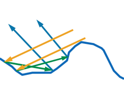
And this effect is called - retroreflection . All these micrograin describes the roughness coefficient ( roughness ), which is usually (but not always) in the range (0;. 1] At 0 we surface is perfectly smooth, and micrograin no At 1 micrograin distributed so that equiprobably reflect light over the hemisphere. Sometimes, the roughness coefficient is replaced by a smoothness coefficient, which is equal to 1-roughness.
That's basically all how surfaces behave for reflected light.
2.2 Bidirectional Reflectance Distribution Function
So, the light entering the surface is partially reflected, and partially penetrates into the material. Therefore, the amount of reflected light is first isolated from the total light flux. Moreover, we are interested not only in the amount of reflected light, but also in the amount of light that enters our eyes. And this is described by various Bidirectional Reflectance Distribution Function (BRDF) .
We will consider one of the most popular models - the Cook-Torrance model :

In this function:
V - vector from the surface to the eye of the observer
N - macro-normal of the surface
L - direction from the surface to the light source
D- the distribution function of reflected light, taking into account micro faces. Describes the number of micro-faces turned towards us so as to reflect light into our eyes.
G is the distribution function of self-shadowing and self-overlapping. Unfortunately, light reflected several times in this function is not taken into account, and will be lost. We will come back to this point later in the article.
F - Fresnel reflection coefficients. Not all light is reflected. Part of the light is refracted and gets into the material. In this function, F describes the amount of reflected light.
Even in the formula, such a parameter as the H vector is not visible , but it will be actively used in the D and G distribution functions. Meaning hvectors - describe the normal micro-faces that contribute to reflected light. Those. a ray of light incident on a micro facet with a normal H will always be reflected in our eyes. Since the angle of incidence is equal to the angle of reflection, we can always calculate H as normalize (V + L) . Something like this:
The distribution functions D and G are an approximate solution, and there are many, and different. At the end of the article I will leave a reference to the list of such distributions. We will use the GGX distribution functions developed by Bruce Walter.
2.3 G. Overlap geometry
Let's start with self-shadowing and overlapping. This feature is the G . The GGX distribution of this function uses the Smith method (Smith 1967, "Geometrical shadowing of a random rough surface"). The main point of this method is that the amount of light lost from the light to the surface and from the surface to the observer will be symmetrical with respect to the macronormal of the damage. Therefore, the function of G , we can be divided into 2 parts, the first half and count the lost light from the angle between N and of L , and then use the same function to calculate the lost light from the angle between V and N . Here is one half of such a function G and describes the distribution of GGX:
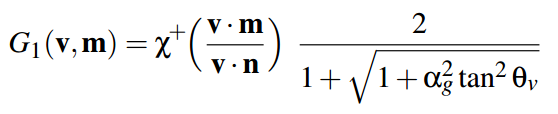
In this function,
α g is the square of the surface roughness (roughness * roughness).
θ v - makronormalyu angle between N and in one case light L , in another case, the vector of the observer V .
Χ - a function that returns zero if the beam under test comes from the opposite side of the normal, in other cases it returns one. In the HLSL shader, we will remove this from the formula, because We’ll check at the earliest stages, and don’t light such a pixel at all. In the original formula, we have the tangent, but for rendering it is convenient to use the cosine of the angle, because we get it through the scalar product. Therefore, I slightly transformed the formula, and wrote it in the HLSL code:
floatGGX_PartialGeometry(float cosThetaN, float alpha){
    float cosTheta_sqr = saturate(cosThetaN*cosThetaN);
    float tan2 = ( 1 - cosTheta_sqr ) / cosTheta_sqr;
    float GP = 2 / ( 1 + sqrt( 1 + alpha * alpha * tan2 ) );
    return GP;
}
And we consider the total G from the light vector and the observer vector as follows:
float roug_sqr = roughness*roughness;
float G = GGX_PartialGeometry(dot(N,V), roug_sqr) * GGX_PartialGeometry(dot(N,L), roug_sqr);
If we render the balls and derive this G , we get something like this:
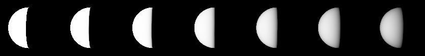
The light source is on the left. The roughness of the balls from left to right is from 0.05 to 1.0.
Check : No pixel should be more than one. Put this condition:
Out.Color = G;
if (Out.Color.r > 1.000001) Out.Color.gb = 0.0;
If at least one output pixel is more than one, then it will turn red. If everything is done correctly, all pixels will remain white.
2.4 D. Distribution of reflective micro facets
So we have such parameters: macronormal , roughness , and H vector. Of these parameters can be set at any% micrograin given pixel have normal coincident with H . In GGX is responsible for it's the function:
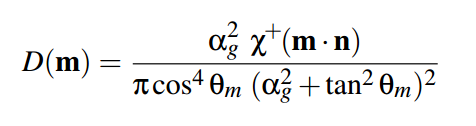
X - the same function as in the case of the G . We throw it away for the same reasons.
α g is the square of the surface roughness;
θ m is the angle between the macro normal N and our H vector.
Again I made some small transformations, and replaced the tangent with the cosine of the angle. As a result, we have just such an HLSL function:
floatGGX_Distribution(float cosThetaNH, float alpha){
    float alpha2 = alpha * alpha;
    float NH_sqr = saturate(cosThetaNH * cosThetaNH);
    float den = NH_sqr * alpha2 + (1.0 - NH_sqr);
    return alpha2 / ( PI * den * den );
}
And call it like this:
float D = GGX_Distribution(dot(N,H), roughness*roughness);If you display the value of D on the screen, we get something like this: The

roughness still changes from 0.05 on the left, to 1.0 on the right.
Check : Please note that with a roughness of 1.0, all light should be distributed evenly throughout the hemisphere. This means that the last ball must be solid. Its color should be 153 153 153 (+ -1 due to rounding), which when converted from sRGB to linear space will give 0.318546778125092. Multiplying this number by PI we should get about one, which corresponds to the reflection in the hemisphere. Why PI? Because the hemisphere integral cos (x) sin (x) gives PI.
2.5 F. Fresnel reflection coefficients
A ray of light, having hit the border of two different media, is reflected and refracted.
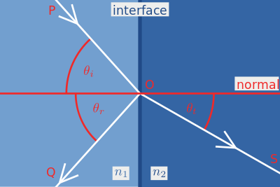
Fresnel formulas accurately describe the laws by which this happens, but if you go to the wiki and look at these multi-story formulas, you will see that they are heavy. Fortunately, there is a good approximation that is used in most cases in PBR renderings, this is the Schlick approximation :

Where R0 is calculated as the ratio of refractive indices:
and cosθ in the formula is the cosine of the angle between the incident light and the normal. It can be seen that for cosθ = 1 the formula degenerates in R0 , which means that the physical meaning of R0- the amount of reflected light if the beam falls perpendicular to the surface. Let's get this straight into hlsl code:
float3 FresnelSchlick(float3 F0, float cosTheta){
    return F0 + (1.0 - F0) * pow(1.0 - saturate(cosTheta), 5.0);
}
Note that F0 is of type float3 . This is due to the fact that the reflection coefficients may be different for different channels. Different materials reflect different amounts of light depending on the wavelength:
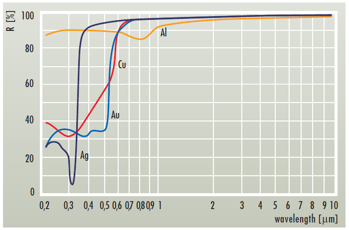
And since we have RGB cones in our eyes, float3 will be enough for people.
2.6 Fold together
Well. Let's now assemble our function that returns the entire reflected color:
float3 CookTorrance_GGX(float3 n, float3 l, float3 v, Material_pbr m){
    n = normalize(n);
    v = normalize(v);
    l = normalize(l);
    float3 h = normalize(v+l);
    //precompute dotsfloat NL = dot(n, l);
    if (NL <= 0.0) return0.0;
    float NV = dot(n, v);
    if (NV <= 0.0) return0.0;
    float NH = dot(n, h);
    float HV = dot(h, v);
    //precompute roughness squarefloat roug_sqr = m.roughness*m.roughness;
    //calc coefficientsfloat G = GGX_PartialGeometry(NV, roug_sqr) * GGX_PartialGeometry(NL, roug_sqr);
    float D = GGX_Distribution(NH, roug_sqr);
    float3 F = FresnelSchlick(m.f0, HV);
    //mix
    float3 specK = G*D*F*0.25/NV;
    return max(0.0, specK);
}
At the very beginning, we filter the light that does not reach the surface:
if (NL <= 0.0) return0.0;if (NV <= 0.0) return0.0;Note that I did not divide by NL:
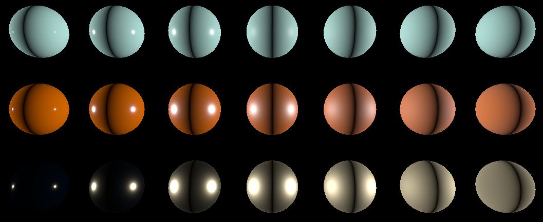
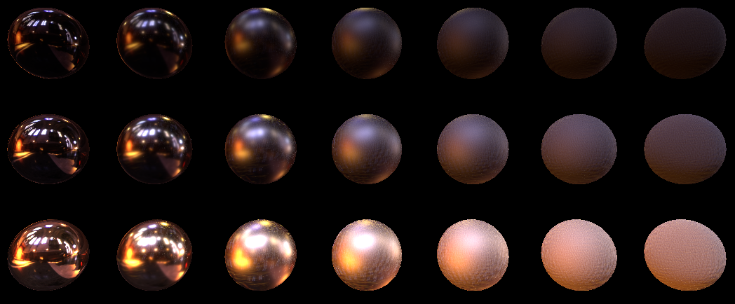
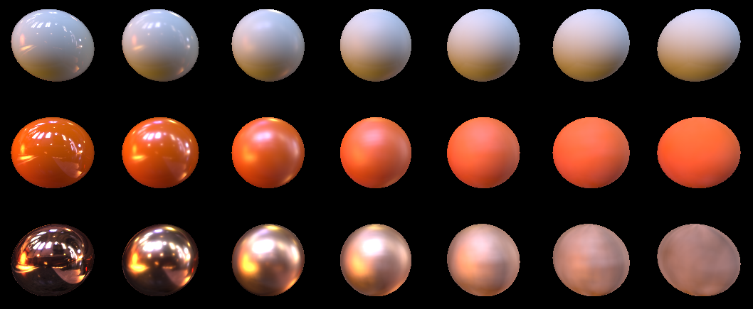
float3 specK = G*D*F*0.25/NV;because then we multiply by NL anyway , and NL is reduced. At the output, I got this picture:
From left to right, the roughness increases from 0.05 to 1.0
From top to bottom, different Fresnel coefficients F0 :
1. (0.04, 0.04, 0.04)
2. (0.24, 0.24, 0.24)
3. (1.0, 0.86, 0.56 )
2.7 Lambertian ambient light model
So the FresnelSchlick function will return us the amount of reflected light. The rest of the light will be equal to 1.0-FresnelSchlick () .
Here I want to make a digression.
Вот эту единицу минус френель многие считают по разному. Например в UE4 FresnelSchlick считают от dot(V,H). Где-то берут два коэффициента (от dot(L,N) и dot(V,N)). Как по мне — логичнее брать от dot(L,N). Сейчас я могу сказать, что я не знаю точно, как правильнее, и как будет ближе к реальности. Когда я изучу этот вопрос, я дополню этот пробел в статье, а пока мы будем делать так, как в UE4, то есть dot(V,H).
This light will pass through the surface and will randomly wander inside it until it is absorbed / reradiated / leaves the surface at another point. Since we are not yet affecting subsurface scattering, we will roughly assume that this light will be absorbed or reradiated in the hemisphere:
In the first approximation, this will suit us. This dispersion is described by the Lambert lighting model . This is described by the simplest formula LightColor * dot (N, L) / PI . That is, familiar to everyone is dot (N, L) , which describes the density of the light flux incident on the surface, and the division by PI , which we have met before in the form of an integral hemisphere . The amount of absorbed / re-emitted light describesfloat3 is a parameter called albedo . Everything here is very similar with the F0 parameter. The subject re-emits only certain wavelengths.
Since Lambert has nothing more to say about the lighting model, we are adding it to our CookTorrance_GGX (although it might have been more correct to put it into a separate function, but I'm too lazy to pull out the F parameter so far):
    float3 specK = G*D*F*0.25/(NV+0.001);
    float3 diffK = saturate(1.0-F);
    return max(0.0, m.albedo*diffK*NL/PI + specK);
But in general, the function has become like this
float3 CookTorrance_GGX(float3 n, float3 l, float3 v, Material_pbr m){
n = normalize(n);
v = normalize(v);
l = normalize(l);
float3 h = normalize(v+l);
//precompute dotsfloat NL = dot(n, l);
if (NL <= 0.0) return0.0;
float NV = dot(n, v);
if (NV <= 0.0) return0.0;
float NH = dot(n, h);
float HV = dot(h, v);
//precompute roughness squarefloat roug_sqr = m.roughness*m.roughness;
//calc coefficientsfloat G = GGX_PartialGeometry(NV, roug_sqr) * GGX_PartialGeometry(NL, roug_sqr);
float D = GGX_Distribution(NH, roug_sqr);
float3 F = FresnelSchlick(m.f0, HV);
//mix
float3 specK = G*D*F*0.25/(NV+0.001);
float3 diffK = saturate(1.0-F);
return max(0.0, m.albedo*diffK*NL/PI + specK);
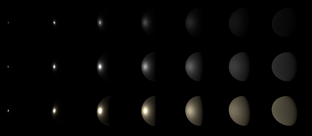
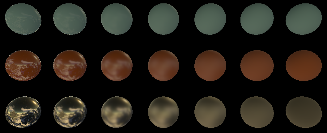
}Here's what I got after adding a diffuse component:
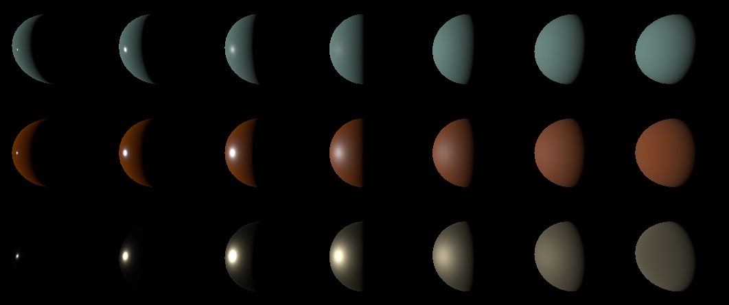
Albedo of three materials (in linear space) from top to bottom:
1. (0.47, 0.78, 0.73)
2. (0.86, 0.176, 0)
3. (0.01, 0.01, 0.01)
Well and so I put the second light source on the right, and increased the intensity of the sources 3 times: The
current example can be downloaded here in the repository. I also remind you that the collected versions of the examples are here .
3.0 Image based lighting
We have now examined how a point source of light contributes to the illumination of each pixel in an image. Of course, we neglected the fact that the source must attenuate from the square of the distance, as well as the fact that the source cannot be point-like, and all this could be taken into account, but let's look at another approach to lighting. The fact is that all objects around reflect / reemit light, and thereby illuminate the environment. You go to the mirror and see yourself. The reflected light in the mirror was recently re-emitted / reflected by your body, and that is why you see yourself in it. If we want to get beautiful reflections in smooth objects, then for each pixel we will need to calculate the light from the hemisphere surrounding this pixel. In games, this fake is used in this case. Prepare a large texture with the environment (actually 360 ° photo or a cubic map). Each pixel of such a photograph is a small emitter. Then, using “some magic”, we select pixels from such textures, and illuminate the pixel being drawn using the code that we wrote above for point sources. That is why the technique is called Image based lighting (i.e., the texture of the environment is used as a light source).
3.1 Monte-Carlo
Let's start with a simple one. We will use the Monte Carlo method to calculate our coverage. For those who are afraid and do not understand the scary words “Monte Carlo method” I’ll try to explain on my fingers. The lighting of each point is affected by all points from the map. We can weed out half of them. These are those that are on the opposite side of the surface, as they will give zero contribution to lighting. We still have a hemisphere. Now we can let out randomly evenly distributed rays in this hemisphere, and stack the lighting in a heap, and then divide by the number of rays emitted and multiply by 2π. At 2π, this is the area of a hemisphere with a radius of 1. Mathematicians will say that we integrated the lighting over the hemisphere using the Monte Carlo method.
How will this work in practice? We will add to the heap using a render in a floating point texture through additive blending. In the alpha channel of this texture we will record the number of our rays, and in rgb the actual lighting. This will allow us to split color.rgb into color.a and get the final image.
However, additive blending means that objects covered by other objects will begin to shine through the others, as they will be drawn. To avoid this problem, we will use the depth prepass technique. The essence of the technique is that we first draw the objects only into the depth buffer , and then switch the depth test to equal and draw the objects now into the color buffer .
So, then I generate a bunch of rays evenly distributed over the sphere:
functionRandomRay(): TVec3;
var theta, cosphi, sinphi: Single;
begin
  theta := 2 * Pi * Random;
  cosphi := 1 - 2 * Random;
  sinphi := sqrt(1 - min(1.0, sqr(cosphi)));
  Result.x := sinphi * cos(theta);
  Result.y := sinphi * sin(theta);
  Result.z := cosphi;
end;
  SetLength(Result, ACount);
  for i := 0to ACount - 1do
    Result[i] := Vec(RandomRay(), 1.0);
and send this stuff as a constant to this shader:
float3 m_albedo;
float3 m_f0;
float  m_roughness;
staticconstfloat LightInt = 1.0;
#define SamplesCount 1024#define MaxSamplesCount 1024
float4 uLightDirections[MaxSamplesCount];
TextureCube uEnviroment; SamplerState uEnviromentSampler;
PS_Output PS(VS_Output In){
    PS_Output Out;
    Material_pbr m;
    m.albedo = m_albedo;
    m.f0 = m_f0;
    m.roughness = m_roughness;
    float3 MacroNormal = normalize(In.vNorm);
    float3 ViewDir = normalize(-In.vCoord);
    Out.Color.rgb = 0.0;
    [fastopt]
    for (uint i=0; i<SamplesCount; i++){ //складываем освещение всех лучей в кучу
        float3 LightDir = dot(uLightDirections[i].xyz, In.vNorm) < 0 ? -uLightDirections[i].xyz : uLightDirections[i].xyz; //нас интересует только полусфера поэтому переворачиваем луч на 180, если он нам не подходит
        float3 LightColor = uEnviroment.SampleLevel(uEnviromentSampler, mul(LightDir, (float3x3)V_InverseMatrix), 0.0).rgb*LightInt; //по лучу берем семпл из кубической карты (наше окружение)
        Out.Color.rgb += CookTorrance_GGX(MacroNormal, LightDir, ViewDir, m)*LightColor; //и считаем освещение по уже написанной функции для точечного источника
    }
    Out.Color.rgb *= 2*PI; //не забываем умножить на площадь единичной полусферы
    Out.Color.a = SamplesCount; //и складываем количество лучей в альфаканалreturn Out;
}
We start, and we see how our picture for the same balls gradually converges. I used two cubic maps for rendering. Here is for this:
I took a cubic map that came with RenderMonkey. It is called Snow.dds. This is an LDR texture and it is boring. Balls seem more dirty than beautifully lit.
And for this:

I took the HDR Probe from here: www.pauldebevec.com/Probes called Grace Cathedral, San Francisco. She has a dynamic range of as much as 200,000: 1. See what's the difference? Therefore, when you make such lighting in yourself, take an HDR texture right away .
By the way, let's see that the law of conservation of energy is fulfilled. To do this, I
forcefully set the albedo in the shader to 1.0: m.albedo = 1.0;
I set the light to 1.0:
LightColor = 1.0;
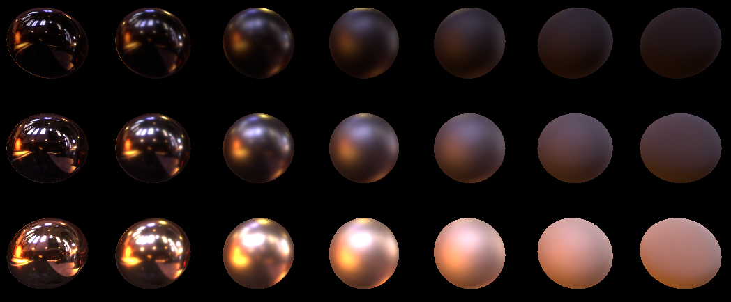
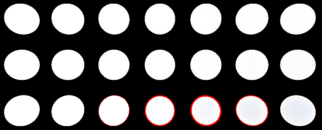
Ideally, each pixel of the ball should now be equal to one. Therefore, everything that goes beyond the unit is marked in red. It happened to me like this:
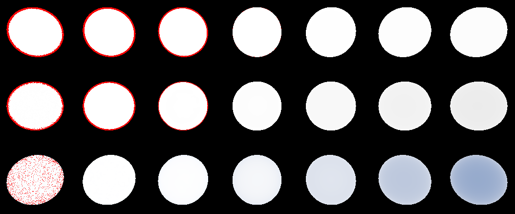
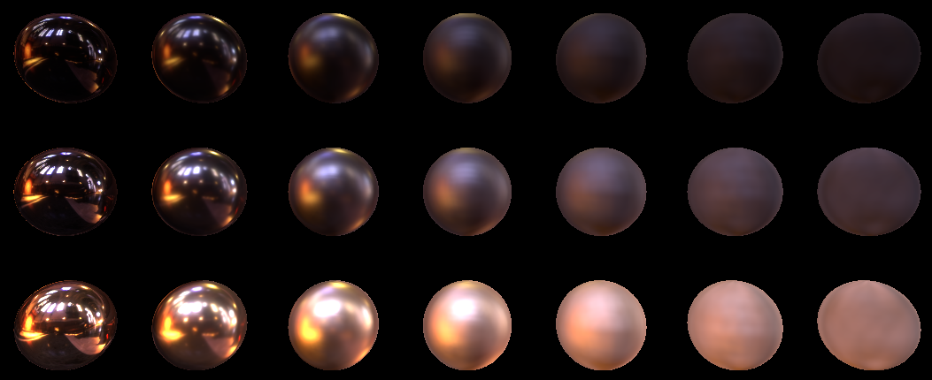
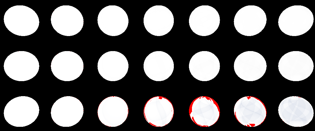
In fact, the red that now exists is errors. It begins to converge, but at some point the accuracy of the float is not enough, and the convergence disappears. Notice that the lower right ball has turned blue. This is because the Lambert model does not take into account surface roughness, and the Cook-Torens model does not take them into account completely. In fact, we have lost the yellow color that goes to F0 . let's tryF0 set all the balls to 1.0 and see: The
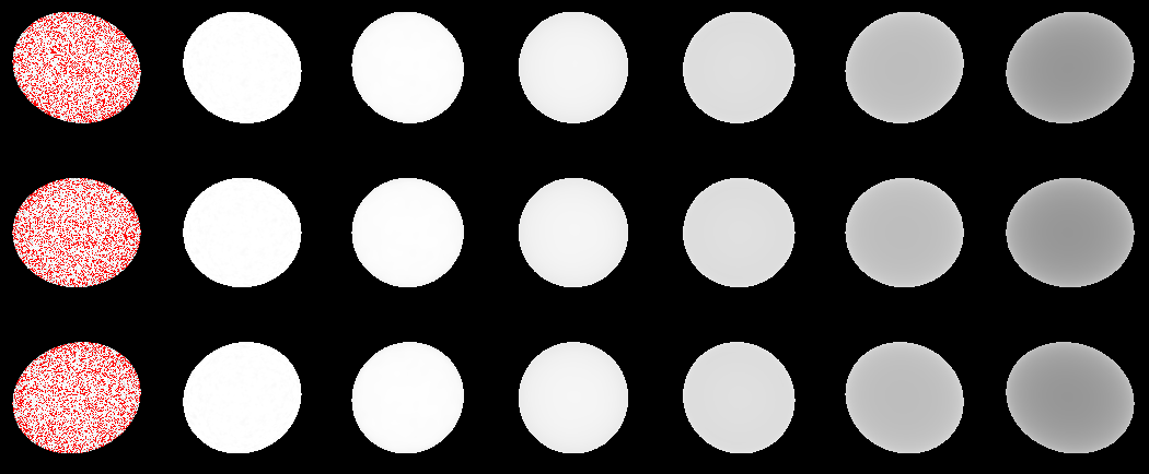
right balls have become much darker due to the large roughness. This is actually a retroreflection that we have lost. Cook Torrens just loses this energy. The Oren-Nayar model can partially restore this energy. But we will postpone it for now. We will have to put up with the fact that for very rough models we will lose up to 70% of the energy of retroreflections.
The source code is here . I already mentioned the collected binaries, they are here .
3.2 Importance sampling
Of course, the gamer will not wait for the light in your picture to converge. Something needs to be done so as not to count the thousands and thousands of rays for each pixel. And the trick is this. For montecarlo, we considered the uniform distribution in the hemisphere. This is how we made the samples:

but the actual part comes from the part circled in pink. If we could choose rays, mainly from the red zone, we would get an acceptable picture much earlier. So we want this:

Fortunately, for this there is a mathematical method called Importance Sampling (or sampling by significance). Significance in our expression contributes parameter D . Using it we can build a CDF (distribution function), from some PDFfunctions (probability density function). For PDF we take the distribution of the micronormal to our normal, the sum in the hemisphere will give one, so we can write such an integral:
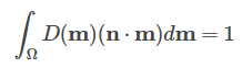
Here is the integrand - PDF
Taking the integral over spherical angles we get this CDF :
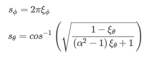
For those who want to go through this step by step stage - you can look here .
For those who do not want / cannot go deeper I will say. We have a CDF into which we substitute evenly distributed ξ , at the output we get a distribution that reflects our PDF . What does this mean for us?
1. That it will change our functionCook Torrens . It will need to be divided into a PDF function.
2. PDF function reflects the distribution of micronormal relative to macronormal. Previously, for Monte Carlo, we took a random vector, and took it as a vector to a light source. Now with the help of CDF , we choose a random vector H . Next, we reflect the gaze vector with respect to this random H and obtain the light vector.
3. Our PDF must be transferred to the space of the form (since it reflects the distribution along the vector N ). To translate, we need to divide our PDF into 4 * dot (H, V) Who cares to delve deeper - gohere and there there are explanations in paragraph 4.1 onwards with drawings in circles.
It seems that nothing is clear, right? Let's try to digest all this in code.
First, write a function that generates a vector H from our CDF . In HLSL, it will be like this:
float3 GGX_Sample(float2 E, float alpha){
    float Phi = 2.0*PI*E.x;
    float cosThetha = saturate(sqrt( (1.0 - E.y) / (1.0 + alpha*alpha * E.y - E.y) ));
    float sinThetha = sqrt( 1.0 - cosThetha*cosThetha);
    return float3(sinThetha*cos(Phi), sinThetha*sin(Phi), cosThetha);
}
Here in E we give a uniform distribution [0; 1) for both spherical angles, in alpha we have the square of the roughness of the material.
At the output, we get an H vector in the hemisphere. But this hemisphere needs to be oriented along the surface. To do this, we write another function that will return to us the orientation matrix on the surface:
float3x3 GetSampleTransform(float3 Normal){
  float3x3 w;
  float3 up = abs(Normal.y) < 0.999 ? float3(0,1,0) : float3(1,0,0);
  w[0] = normalize ( cross( up, Normal ) );
  w[1] = cross( Normal, w[0] );
  w[2] = Normal;
  return w;
}
By this matrix, we will multiply all our generated vectors H , translating their tangent space into a space of the form. The principle is very similar to the TBN basis.
Now it remains to divide our Cook-Torrens: G * D * F * 0.25 / (NV) into PDF . Our PDF = D * NH / (4 * HV) . Therefore, our modified Cook-Torrens turns out:
G * F * HV / (NV * NH)
In HLSL now it looks like this:
float3 CookTorrance_GGX_sample(float3 n, float3 l, float3 v, Material_pbr m, out float3 FK){
    pdf = 0.0;
    FK = 0.0;
    n = normalize(n);
    v = normalize(v);
    l = normalize(l);
    float3 h = normalize(v+l);
    //precompute dotsfloat NL = dot(n, l);
    if (NL <= 0.0) return0.0;
    float NV = dot(n, v);
    if (NV <= 0.0) return0.0;
    float NH = dot(n, h);
    float HV = dot(h, v);
    //precompute roughness squarefloat roug_sqr = m.roughness*m.roughness;
    //calc coefficientsfloat G = GGX_PartialGeometry(NV, roug_sqr) * GGX_PartialGeometry(NL, roug_sqr);
    float3 F = FresnelSchlick(m.f0, HV);
    FK = F;
    float3 specK = G*F*HV/(NV*NH);
    return max(0.0, specK);
}
Please note that I threw out the diffuse part from the Lambert lighting from this function, and I return the FK parameter out. The fact is that we cannot count the diffuse component through Importance Sampling , because our PDF is for faces that reflect light in our eyes. And the Lambert distribution does not depend on this. What to do? Hmm ... for now let’s leave the diffuse part black and focus on the specular.
PS_Output PS(VS_Output In){
    PS_Output Out;
    Material_pbr m;
    m.albedo = m_albedo;
    m.f0 = m_f0;
    m.roughness = m_roughness;
    float3 MacroNormal = normalize(In.vNorm);
    float3 ViewDir = normalize(-In.vCoord);
    float3x3 HTransform = GetSampleTransform(MacroNormal);
    Out.Color.rgb = 0.0;
    float3 specColor = 0.0;
    float3 FK_summ = 0.0;
    for (uint i=0; i<(uint)uSamplesCount; i++){
        float3 H = GGX_Sample(uHammersleyPts[i].xy, m.roughness*m.roughness); //генерим H вектор
        H = mul(H, HTransform); //переводим из пространства модели в пространство вида
        float3 LightDir = reflect(-ViewDir, H); //отражаем вектор взгляда чтобы получить вектор света
        float3 specK;
        float3 FK;
        specK = CookTorrance_GGX_sample(MacroNormal, LightDir, ViewDir, m, FK); //считаем количество спекуляра
        FK_summ += FK;
        float3 LightColor = uRadiance.SampleLevel(uRadianceSampler, mul(LightDir.xyz, (float3x3)V_InverseMatrix), 0).rgb*LightInt;//и множим его на пиксель из карты света
        specColor += specK * LightColor; //добавляем в сумму
    }
    specColor /= uSamplesCount;
    FK_summ /= uSamplesCount;
    Out.Color.rgb = specColor;
    Out.Color.a = 1.0;
    return Out;
}
Let's set 1024 samples (without accumulation like in Monte Carlo) and look at the result:
Although there are a lot of samples, it turned out noisy. Especially at great roughness.
3.3 Choosing LODs
This is because we take samples from a highly detailed map, from zero LOD . And it would be good for rays with a large deviation to take a smaller lod. This picture is well illustrated by this picture:

From this article from NVidia. The blue areas show the average value, which would be nice to take from the LODs of the texture. It can be seen that for the more significant we take a smaller LOD , and for the less significant more, i.e. we take the value averaged over the region. It would be ideal if we covered the entire hemisphere with lodas. Fortunately, NVidia has already given us a ready-made (and simple in their words) formula:

This formula consists of the difference:
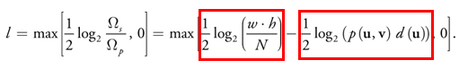
The left part with us depends on the size of the texture and the number of samples. And this means that for all samples we can count it once. On the right side we have the function p , which is nothing but our pdf , and the function d , which they call distortion , but in fact there is a dependence on the angle of the sample to the observer. For d , they have this formula:

Spoiler heading
(Внимание, данная формула справедлива для Dual-Paraboloid карт. У нас используется кубическая карта, и я полагаю, что коэффициент b для нашего случая может быть другой, но я это еще не проверял. В моем случае коэффициент предложенный в статье b=1.2 сработал достаточно неплохо)
Well, NVidia also recommends making bias for lods, adding one. Let's see how it looks in hlsl code. Here is our left side of the equation:
floatComputeLOD_AParam(){
    float w, h;
    uRadiance.GetDimensions(w, h);
    return0.5*log2(w*h/uSamplesCount);
}
Here we consider the right side, and immediately subtract it from the left:
floatComputeLOD(float AParam, float pdf, float3 l){
    float du = 2.0*1.2*(abs(l.z)+1.0);
    return max(0.0, AParam-0.5*log2(pdf*du*du)+1.0);
}
Now we see that we need to pass pdf and l values to us in ComputeLOD . l is the vector of the light sample, and pdf , if we look above, this is ours: pdf = D * dot (N, H) / (4 * dot (H, V)) . Therefore, let's add the return pdf parameter to our CookTorrance_GGX_sample function :
float3 CookTorrance_GGX_sample(float3 n, float3 l, float3 v, Material_pbr m, out float3 FK, out float pdf){
    pdf = 0.0;
    FK = 0.0;
    n = normalize(n);
    v = normalize(v);
    l = normalize(l);
    float3 h = normalize(v+l);
    //precompute dotsfloat NL = dot(n, l);
    if (NL <= 0.0) return0.0;
    float NV = dot(n, v);
    if (NV <= 0.0) return0.0;
    float NH = dot(n, h);
    float HV = dot(h, v);
    //precompute roughness squarefloat roug_sqr = m.roughness*m.roughness;
    //calc coefficientsfloat G = GGX_PartialGeometry(NV, roug_sqr) * GGX_PartialGeometry(NL, roug_sqr);
    float3 F = FresnelSchlick(m.f0, HV);
    FK = F;
    float D = GGX_Distribution(NH, roug_sqr); //вот тут собственно мы добавили вычисление D
    pdf = D*NH/(4.0*HV); //и вычисление самой pdf
    float3 specK = G*F*HV/(NV*NH);
    return max(0.0, specK);
}
And the sample loop itself now calculates the LOD :
float LOD_Aparam = ComputeLOD_AParam();
    for (uint i=0; i<(uint)uSamplesCount; i++){
        float3 H = GGX_Sample(uHammersleyPts[i].xy, m.roughness*m.roughness);
        H = mul(H, HTransform);
        float3 LightDir = reflect(-ViewDir, H);
        float3 specK;
        float pdf;
        float3 FK;
        specK = CookTorrance_GGX_sample(MacroNormal, LightDir, ViewDir, m, FK, pdf);
        FK_summ += FK;
        float LOD = ComputeLOD(LOD_Aparam, pdf, LightDir);
        float3 LightColor = uRadiance.SampleLevel(uRadianceSampler, mul(LightDir.xyz, (float3x3)V_InverseMatrix), LOD).rgb*LightInt;
        specColor += specK * LightColor;
    }
Let's take a look at what we got for 1024 samples with lods:
It looks perfect. Lower to 16, and ...
Yes, of course it’s not quite perfect. It can be seen that the quality suffered on balls with great roughness, but nevertheless I consider this quality acceptable in principle. It would be possible to further improve the quality if we built mip- s for textures based on our distribution. This can be found in the presentation from Epic here (see the Pre-Filtered Environment Map paragraph). In the meantime, as part of this article, I propose to dwell on the classic pyramidal mipes.
3.4 Hammersley point set
If you look at our random rays, then the flaw is clear. They are random. And we have already learned to read from lods and we want to capture as large a square as possible with our rays. To do this, we need to "spray" our rays, but taking into account the importance of sampling. Because Since the CDF takes a uniform distribution, it’s enough for us to evenly distribute the points in the interval [0; 1) ... but we have a uniform distribution should be two-dimensional. Therefore, it is necessary not only to evenly arrange the points in the gap, but also to make the distance in Cartesian coordinates between the points as large as possible. The Hammersley point set is well suited for this role . You can read a little more about this many points here .
I will only show the distribution picture:

I will also give a function that generates a separate point:
functionHammersleyPoint(const I, N: Integer): TVec2;
  functionradicalInverse_VdC(bits: Cardinal): Single;
  begin
    bits := (bits shl16) or (bits shr16);
    bits := ((bits and $55555555) shl1) or ((bits and $AAAAAAAA) shr1);
    bits := ((bits and $33333333) shl2) or ((bits and $CCCCCCCC) shr2);
    bits := ((bits and $0F0F0F0F) shl4) or ((bits and $F0F0F0F0) shr4);
    bits := ((bits and $00FF00FF) shl8) or ((bits and $FF00FF00) shr8);
    Result := bits * 2.3283064365386963e-10;
  end;
begin
  Result.x := I/N;
  Result.y := radicalInverse_VdC(I);
end;
How will our balls look with this set of dots? In fact, I faked, and all the above images for Importance Sampling were generated with a set of these points. On random sets, the pictures look a little worse (believe the word?)
3.5 Irradiance map
Remember how we were left without a diffuse color? We cannot sample diffuse color with importance sampling because our importance sampling selects the most valuable rays for the speculator. For diffusion, the most valuable ones are located directly opposite, on the macro normal surface. Fortunately, the diffuse component for Lambert is completely independent of the observer. Therefore, we can calculate the lighting in a cubic map. And another bonus is that changing the angle affects the lighting so slightly that the calculated map can be of very low resolution, for example 16 * 16 pixels per side.
This time we were lucky. We will not write code that builds the Irradiance map , but use the CubeMapGen program. Just open our cubmap (Load Cubemap (.dds)), set the Irradiance cubemap checkbox, select Output Cube Size 16:
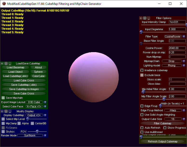
and save the resulting cubic map (for HDR textures, do not forget to set the desired texture output format).
Well, since we figured out the Irradiance map , we simply add one sample from this map after sampling. Our HLSL code now looks like this:
    Out.Color.rgb = 0.0;
    float3 specColor = 0.0;
    float3 FK_summ = 0.0;
    for (uint i=0; i<(uint)uSamplesCount; i++){
        float3 H = GGX_Sample(uHammersleyPts[i].xy, m.roughness*m.roughness);
        H = mul(H, HTransform);
        float3 LightDir = reflect(-ViewDir, H);
        float3 specK;
        float pdf;
        float3 FK;
        specK = CookTorrance_GGX_sample(MacroNormal, LightDir, ViewDir, m, FK, pdf);
        FK_summ += FK;
        float LOD = ComputeLOD(LOD_Aparam, pdf, LightDir);
        float3 LightColor = uRadiance.SampleLevel(uRadianceSampler, mul(LightDir.xyz, (float3x3)V_InverseMatrix), LOD).rgb*LightInt;
        specColor += specK * LightColor;
    }
    specColor /= uSamplesCount;
    FK_summ /= uSamplesCount;
    float3 LightColor = uIrradiance.Sample(uIrradianceSampler, mul(MacroNormal, (float3x3)V_InverseMatrix)).rgb;
    Out.Color.rgb = m.albedo*saturate(1.0-FK_summ)*LightColor + specColor;
And at the output we have this picture for 16 samples:
And such for 1024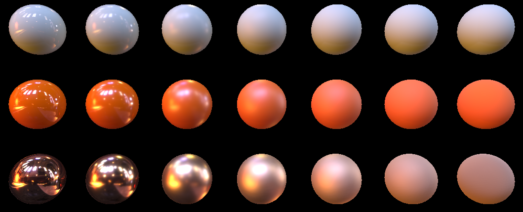
Please note that we no longer multiply diffuse light by dot (N, L) , which is kind of logical. After all, we calculated this lighting and baked it in a cubmap, and in our case N and L are generally the same vector. Let's see what we have there with energy conservation? As usual, we set the light from cubic cards to unity, set the albedo of the material to unity, and highlight areas> 1 in red. We get roughly this for 1024 samples:
And here it is for 16:
As you can see, there are obvious "emissions" of excess energy, but they are small. This is due to the fact that we do not accurately calculate the amount of light from diffuse energy. After all, we consider the Fresnel coefficients only for certain samples of the specular, and use them for all the samples that are calculated in the irradiance map . Alas, I do not know what to do with this, the Internet could not tell me anything. Therefore, I propose for now to come to terms with this, all the same, the emissions of excess energy are not significant.
4 A little more about the materials.
While we were messing around with the balls - you should have noticed that we have two float3 color options. This is albedo and f0 . They both have some physical meaning, but in games, as a rule, materials are divided into metals and non-metals. The fact is that non-metals always reflect light in the grayscale ranges, but at the same time re-emit the light of color. Metals, on the contrary, reflect colored light, but at the same time absorb the rest.
That is, for metals we have:
albedo = {0, 0, 0}
f0 = {R, G, B}
for our dielectrics:
albedo = {R, G, B}
f0 = {X, X, X}
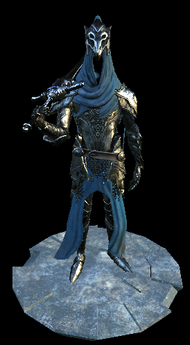
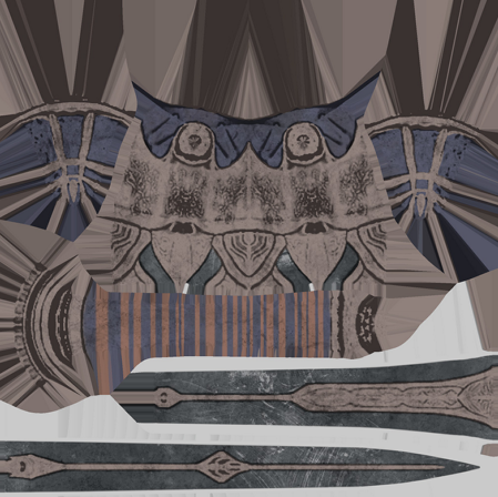
and ... we see that we can introduce a certain coefficient [0,1], by which we will show how much our surface is metallic, and consider the material simply through linear interpolation. This is actually many artists do. I downloaded this 3d model.
Here's an example of a sword texture.
Texture of color:
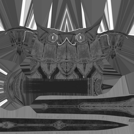
Texture of roughness:
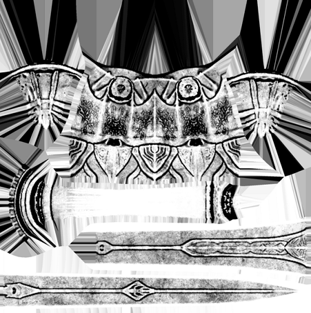
And finally, the texture of metallicity (the one I mentioned above):
You can read a little more about the materials on the Internet. For example here .
Different engines and studios can pack parameters in different ways, but as a rule, everything revolves around: color, roughness, metallicity.
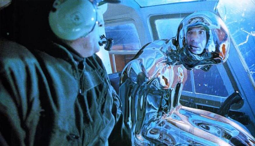
And finally, how it looks on the whole model:
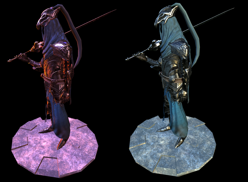
on the left is the same cathedral that we tested on balls. On the right, our Artorias got out into the nature (the environment map from here www.pauldebevec.com/Probes is called Campus).
To render these images, I additionally used Reinhard tonmapping, but this topic is already for a separate article.
The source code for the Artorias model is a demo in my framework, and is located here . I also put together a version for you, and uploaded it here .
5 Conclusion
The article came out much more than I expected. I would like to tell you more about:
1. Anisotropic lighting models
2. Subsurface scattering
3. Advanced diffuse lighting models, such as Oren-Nayar
4. Capture spherical harmonics
5. Capture tonmapping
But believe it or not, I was exhausted while writing this article ... And here everyone point is a thick layer. Therefore, there is, that is. Maybe someday I’ll talk about all this.
I hope that my article will reveal to someone the veil of secrecy hidden behind these letters PBR. And thanks for watching.
Useful PBR and so on
[1] blog.tobias-franke.eu/2014/03/30/notes_on_importance_sampling.html
откуда взялись PDF и CDF, и как их посчитать самому.
[2] hal.inria.fr/hal-00942452v1/document
хороший математический материал по PBR (+ анизотропные распределения)
[3] disney-animation.s3.amazonaws.com/library/s2012_pbs_disney_brdf_notes_v2.pdf
хороший материал от Disney, что как можно запаковать и предрасчитать. Сравнение погрешностей, а так же пример нескольких диффузных моделей освещения
[4] blog.selfshadow.com/publications/s2015-shading-course/#course_content
И еще более свежий материал от Disney
[5] www.cs.cornell.edu/~srm/publications/EGSR07-btdf.pdf
Подробно о GGX, от Bruce Walter-а и других умных ребят
[6] de45xmedrsdbp.cloudfront.net/Resources/files/2013SiggraphPresentationsNotes-26915738.pdf
Про PBR в Unreal Engine 4
[7] holger.dammertz.org/stuff/notes_HammersleyOnHemisphere.html
Классная инструкция по Hammersley Point Set
[8] www.jordanstevenstechart.com/physically-based-rendering
Различные функции распределения. С картиночками.
[9] graphicrants.blogspot.nl/2013/08/specular-brdf-reference.html
еще функции распределения
[10] developer.nvidia.com/gpugems/GPUGems3/gpugems3_ch20.html
Очень полезный материал от NVidia про Importance Sampling и оптимизацию LOD-ами.
[11] cgg.mff.cuni.cz/~jaroslav/papers/2008-egsr-fis/2008-egsr-fis-final-embedded.pdf
Еще один неплохой пейпер про Importance Sampling
[12] gdcvault.com/play/1024478/PBR-Diffuse-Lighting-for-GGX
Просто очень качественные слайды по PBR.
[13] www.codinglabs.net/article_physically_based_rendering.aspx
[14] www.codinglabs.net/article_physically_based_rendering_cook_torrance.aspx
Две очень хорошие для понимания основ статьи (но содержат кое-какие ошибки и неточности)
[15] www.rorydriscoll.com/2009/01/25/energy-conservation-in-games
Про сохранение энергии
[16] www.gamedev.net/topic/625981-lambert-and-the-division-by-pi
www.wolframalpha.com/input/?i=integrate+cos+x+*+sin+x+dx+dy+from+x+%3D+0+to+pi+%2F+2+y+%3D+0+to+pi+*+2
откуда Пи в знаменателе
[17]https://seblagarde.files.wordpress.com/2015/07/course_notes_moving_frostbite_to_pbr_v32.pdf
[18] www.pauldebevec.com/Probes
Набор HDR 360 проб. Прямо с формулами как читать из этих проб.
[19] seblagarde.wordpress.com/2012/06/10/amd-cubemapgen-for-physically-based-rendering
code.google.com/archive/p/cubemapgen/downloads
КубМапГен. Тулза для обработки radiance и irradiance кубических карт.
[20] eheitzresearch.wordpress.com/415-2
Про полигональные источники света. С демкой.