Noise Functions and Card Generation
- Transfer

When I studied audio processing, my brain began to draw analogies with procedural card generation. The article outlines the principles linking signal processing with card generation. I don’t think that I discovered something new, but some of the conclusions were new to me, so I decided to write them down and share them with readers. I consider only simple topics (frequency, amplitude, noise colors, noise use) and do not touch on other topics (discrete and continuous functions, FIR / IIR filters, fast Fourier transform, complex numbers). The mathematics of the article is mainly related to sinusoids.
This article focuses on concepts ranging from the simplest to the most complex. If you want to go straight to generating terrain using noise functions, then check out my other article.
I'll start with the basics of using random numbers, and then move on to explain the work of one-dimensional landscapes. The same concepts work for 2D (see demo ) and 3D. Try moving the slider [in the original article] to see how a single parameter can describe different types of noise:
GIF
From this article you will learn:
- how to generate similar landscapes in just 15 lines of code
- what is red, pink, white, blue and purple noise
- how can noise functions be used for procedural card generation
- how midpoint offset, Perlin noise, and fractal Brownian motion are applied
In addition, I will conduct experiments with 2D noise, including creating a 3D visualization of a two-dimensional height map.
1. Why is randomness useful?
We need the procedural generation of maps to obtain sets of output data that have something in common and something different. For example, all Minecraft maps have a lot in common: biome areas, grid size, average size of biomes, heights, average size of caves, percentage of each type of stone, etc. But they also have differences: the location of biomes, the location and shape of caves, the placement of gold, and more. As a designer, you need to decide which aspects should remain the same and which should be different, and take the degree of this difference.
For different aspects, we usually use a random number generator. Let's create an ultra-simple card generator: it will generate lines of 20 blocks, and one of the blocks will contain a chest of gold. Let's describe a few cards that we need (a treasure is marked with an “x”):
карта 1 ........x...........
карта 2 ...............x....
карта 3 .x..................
карта 4 ......x.............
карта 5 ..............x.....
Notice how much these cards have in common: they all consist of blocks, blocks are on the same line, the line has a length of 20 blocks, there are two types of blocks and exactly one treasure chest.
But there is one different aspect - the location of the block. It can be in any position, from 0 (left) to 19 (right).
We can use a random number to select the position of this block. The easiest way is to use a uniform choice of a random number from the range from 0 to 19. This means that the probability of choosing any position from 0 to 19 is the same. Most programming languages have functions for uniformly generating random numbers. In Python, this is a function
random.randint(0,19), but in the article we will use the notation random(0,19). Here is a sample Python code:def gen():
map = [0] * 20 # создаём пустую карту
pos = random.randint(0, 19) # выбираем точку
map[pos] = 1 # помещаем туда сокровище
return map
for i in range(5): # создаём 5 разных карт
print_chart(i, gen())But suppose we need a chest that is more likely to be on the left on maps. To do this, we need a heterogeneous selection of random numbers. There are many ways to implement it. One of them is to choose a random number in a uniform way, and then shift it to the left. For example, you can try
random(0,19)/2. Here is the Python code for this:def gen():
map = [0] * 20
pos = random.randint(0, 19) // 2
map[pos] = 1
return map
for i in range(5):
print_chart(i, gen())But actually I didn’t want this at all. I wanted treasures sometimes to the right, but more often to the left. Another way to move the treasures to the left is to square the number by doing something like
sqr(random(0,19))/19. If it is zero, then 0 squared, divided by 20, is 0. If it is 19, then 19 squared, divided by 19, will be 19. But in the interval, if the number is 10, then 10 squared, divided by 19, equal to 5. We kept the range from 0 to 19, but moved the intermediate numbers to the left. This redistribution in itself is a very useful technique, in previous projects I used squares, square roots and other functions. (On this siteThere are standard form-changing functions used in animations. Hover over the function to see the demo.) Here is the Python code for using squaring:def gen():
map = [0] * 20
pos = random.randint(0, 19)
pos = int(pos * pos / 19)
map[pos] = 1
return map
for i in range(1, 6):
print_chart(i, gen())Another way to move objects to the left is to first randomly select the limit of the range of random numbers, then randomly select a number from 0 to the limit of the range. If the range limit is 19, then we can put the number anywhere. If the range limit is 10, then numbers can only be placed on the left side. Here is the Python code:
def gen():
    map = [0] * 20
    limit = random.randint(0, 19)
    pos = random.randint(0, limit)
    map[pos] = 1
    return map
for i in range(5):
    print_chart(i, gen())
There are many ways to obtain uniform random numbers and turn them into heterogeneous, having the desired properties. As a game designer, you can choose any distribution of random numbers. I wrote an article on how to use random numbers to determine damage in role-playing games. There are various examples of tricks.
Summarize:
- For procedural generation, we need to decide what will remain the same and what will change.
- Random numbers are useful for filling in changing parts.
- Uniformly selectable random numbers can be obtained in most programming languages, but often we need heterogeneous selectable random numbers. There are different ways to get them.
2. What is noise?
Noise is a series of random numbers usually located on a line or in a grid.
When switching to a channel without a signal on old TVs, we saw random black and white dots on the screen. This is noise (their outer space!). When tuning to a radio channel without a station, we also hear noise (not sure if it appears from space, or from somewhere else).
When processing signals, noise is usually an undesirable aspect. In a noisy room it’s harder to hear someone you’re talking to than in a quiet room. Audio noise is random numbers lined up in a line (1D). On a noisy image, it’s harder to see a picture than on a clear image. Graphic noise is random numbers located in a grid (2D). You can create noise in 3D, 4D, and so on.
Although in most cases we try to get rid of noise, many natural systems look noisy, so to generate something that looks like natural, we need to add noise. Although real systems look noisy, they are usually based on structure. The noise we add will not have the same structure, but it is much simpler than programming the simulation, so we use noise, and we hope that the end user will not notice this. I will talk about this compromise later.
Let's look at a simple example of the usefulness of noise. Suppose we have a one-dimensional map, which we made above, but instead of one treasure chest, we need to create a landscape with valleys, hills and mountains. Let's start by using a uniform selection of random numbers at each point. If
random(1,3)equal to 1, we will consider it a valley, if 2 - hills, if 3 - mountains. I used random numbers to create a height map: for each point in the array, I saved the height of the terrain. Here is the Python code for creating the landscape:for i in range(5):
random.seed(i) # даёт каждый раз одинаковые результаты
print_chart(i, [random.randint(1, 3)
for i in range(mapsize)])
# примечание: я использую синтаксис генератора списков Python:
# output = [abc for x in def]
# это упрощённая запись такого кода:
# output = []
# for x in def:
# output.append(abc)Hmm, these cards look "too random" for our purposes. Perhaps we need larger areas of valleys or hills, and mountains should not be as frequent as valleys. Earlier we saw that a uniform choice of random numbers may not be suitable for us, sometimes we need a heterogeneous choice. How to solve this problem? You can use some random choice in which valleys appear more often than mountains:
for i in range(5):
    random.seed(i)
    print_chart(i, [random.randint(1, random.randint(1, 3))
                    for i in range(mapsize)])
This reduces the number of mountains, but does not create any interesting drawings. The problem with such a heterogeneous random choice is that the changes occur at each point separately, and we need the random choice at one point to be somehow related to random choices at neighboring points. This is called coherence.
And here noise functions are useful to us. They give us a set of random numbers instead of one number at a time. Here we need a 1D noise function to create a sequence. Let's try to use a noise function that changes the sequence of homogeneous random numbers. There are different ways to do this, but we use a minimum of two adjacent numbers. If the initial noise is 1, 5, 2, then the minimum (1, 5) is 1, and the minimum (5, 2) is 2. Therefore, the final noise will be 1, 2. Note that we eliminated the high point (5). Also note that in the resulting noise, one value is less than the original. This means that when generating 60 random numbers, the output will be only 59. Let's apply this function to the first set of cards:
def adjacent_min(noise):
    output = []
    for i in range(len(noise) - 1):
        output.append(min(noise[i], noise[i+1]))
    return output
for i in range(5):
    random.seed(i)
    noise = [random.randint(1, 3) for i in range(mapsize)]
    print_chart(i, adjacent_min(noise))
Compared to the previous maps, here we have obtained areas of valleys, hills or mountains. Mountains more often appear near the hills. And thanks to the method of changing noise (choosing a minimum), valleys are more common than mountains. If we took the maximum, the picture would be the opposite. If we wanted neither the valleys nor the mountains to be frequent, we would choose the average instead of the minimum or maximum.
Now we have a noise modification procedure that receives noise at the input and creates a new, smoother noise.
And let's try to run it again!
def adjacent_min(noise):  # так же как раньше
    output = []
    for i in range(len(noise) - 1):
        output.append(min(noise[i], noise[i+1]))
    return output
for i in range(5):
    random.seed(i)
    noise = [random.randint(1, 3) for i in range(mapsize)]
    print_chart(i, adjacent_min(adjacent_min(noise)))
Now the maps have become even smoother and they have even fewer mountains. I think we have smoothed out too much, because mountains do not appear with hills too often. Therefore, it is probably better to go back one level of smoothing in this example.
This is a standard process for procedural generation: you try something, see if it looks good, if not, come back and try something else.
Note: anti-aliasing in signal processing is called a low-pass filter . Sometimes it is used to eliminate unnecessary noise.
Summarize:
- Noise is a set of random numbers, usually lined up in a line or grid.
- In procedural generation, you often need to add noise to create variations.
- A simple choice of random numbers (whether it is homogeneous or heterogeneous) leads to noise, in which each number is not connected with those around it.
- Often we need noise with certain characteristics, for example, getting mountains near the hills.
- There are many ways to make noise.
- Some noise functions create noise directly; others take existing noise and modify it.
The selection of the noise function is often a trial and error process. Understanding the essence of noise and how to modify it allows you to make a more meaningful choice.
3. Making noise
In the previous section, we selected noise using random numbers as the output, and then smoothed them. This is a standard pattern: start with a noise function that uses random numbers as parameters . We used it when a random number chose the position of the treasure, and then we used another where random numbers chose valleys / hills / mountains. You can modify the existing noise to change its shape according to the requirements. We modified the valleys / hills / mountains noise function by smoothing it. There are many different ways to modify noise functions.
Examples of simple 1D / 2D noise generators:
- Use random numbers directly for output. So we did for valleys / hills / mountains.
- Use random numbers as parameters for sines and cosines, which are used for output.
- Use random numbers as parameters for gradients that are used for output. This principle is used in Perlin's noise.
Here are some common ways to modify noise:
- Apply a filter to reduce or enhance certain characteristics. For valleys / hills / mountains, we used anti-aliasing to reduce jumps, increase the areas of the valleys and create mountains near the hills.
- Add several noise functions at the same time, usually with a weighted sum so that you can control the effect of each noise function on the final result.
- Interpolate between the noise values obtained by the noise function to generate smoothed areas.
There are so many ways to make noise!
To some extent, it doesn't matter how the noise was made. This is interesting, but when using the game you need to focus on two aspects:
- How will you use the noise?
- What properties do you need from the noise function in each case?
4. Ways to use noise
The most straightforward way to use the noise function is to use it directly as a height. In the example above, I generated valleys / hills / mountains, calling
random(1,3)maps at every point. The noise value is directly used as height. The use of midpoint displacement noise or Perlin noise are also examples of direct use.
Another way to use noise is to use it as an offset from the previous value. For example, if the noise function returns
[2, -1, 5], then we can assume that the first position is 2, the second is 2 + -1 = 1, and the third is 1 + 5 = 6. See also “random walk” . You can do the opposite, and use the difference between the noise values. This can also be taken as a modification of the noise function.Instead of using noise to set heights, you can use it for audio.
Or to create forms. For example, you can use noise as the radius of the graph in polar coordinates. You can convert a 1D noise function, such as this one, to a polar form, using the output as a radius rather than a height. It shows how the same function looks in polar form.
Or you can use noise as a graphic texture. Perlin noise is often used for this purpose.
You can apply noise to select locations for objects, such as trees, gold mines, volcanoes, or earthquake cracks. In the example above, I used a random number to select the location of the treasure chest.
You can also use noise as a thresholdfunction. For example, you can assume that at any time when the value is above 3, one event occurs, otherwise something else happens. One example of this is using Perlin's 3D noise to generate caves. It can be accepted that everything is above a certain threshold of density, and everything below this threshold is open air (cave).
In my polygon map generator, I used various ways to use noise, but in none of them noise was used directly to determine the height:
- The graph structure is easiest when using a grid of squares or hexagons (in fact, I started with a grid of hexagons). Each grid element is a polygon. I wanted to add randomness to the grid. This can be done by moving points randomly. But I needed something more random. I used a blue noise generator to place polygons and a Voronoi diagram for out reconstruction. It would have taken a lot more time, but, fortunately, I had a library (
as3delaunay) that did everything for me. But I started with the grid, which is much simpler, and it is with it that I recommend starting with you. - The coastline is a way to separate land from water. I used two different ways to generate it using this noise, but you can also ask the designer to draw the shape myself, and I demonstrated it using square and round shapes. The radial shape of the coastline is a noise function using sines and cosines, rendering them in polar form. Perlin's coastline shape is a noise generator that uses Perlin noise and radial return as a threshold. Any number of noise functions can be used here.
- The sources of the rivers are randomly located.
- The boundaries between polygons change from straight lines to noisy lines. This is similar to midpoint displacement, but I scaled them to fit within polygon boundaries. This is a purely graphic effect, so the code is in the GUI (
mapgen.as) instead of the underlying algorithm (Map.as).
Most manuals use noise fairly straightforwardly, but there are many more different ways to use it.
5. Noise frequency
Frequency is the most important property that we are interested in. The easiest way to understand it is to look at the sinusoids. Here is a sine wave with a low frequency, after it there is a sine wave with an average frequency, and at the end there is a sine wave with a high frequency:
print_chart(0, [math.sin(i*0.293) for i in range(mapsize)])print_chart(0, [math.sin(i*0.511) for i in range(mapsize)])print_chart(0, [math.sin(i*1.57) for i in range(mapsize)])As you can see, low frequencies create wide hills, and high frequencies create narrower ones. Frequency describes the horizontal size of the graph; amplitude describes the vertical size. Remember, I said earlier that the maps of valleys / hills / mountains look “too random” and wanted to create wider areas of valleys or mountains? In fact, I needed a low frequency of variation.
If you have a continuous function, for example,
sinthat creates noise, then increasing the frequency means multiplying the input data by some factor: it sin(2*x)will double the frequency sin(x). Increasing the amplitude means multiplying the output by a factor: 2*sin(x)doubles the amplitudesin(x). The code above shows that I changed the frequency by multiplying the input by different numbers. We use the amplitude in the next section when summing several sinusoids.Frequency change
Amplitude change
All of the above applies to 1D, but the same thing happens in 2D. Take a look at Figure 1 on this page . You see examples of 2D noise with a long wavelength (low frequency) and a small wavelength (high frequency). Note that the higher the frequency, the smaller the individual fragments.
When talking about the frequency, wavelength or octave of the noise functions, this is exactly what is meant, even if sinusoids are not used.
Speaking of sinusoids, you can do funny things by combining them in strange ways. For example, here are the low frequencies on the left and the high frequencies on the right:
print_chart(0, [math.sin(0.2 + (i * 0.08) * math.cos(0.4 + i*0.3))
                for i in range(mapsize)])
Usually at the same time you will have many frequencies, and no one will give the correct answers about the choice of the one you need. Ask yourself: what frequencies do I need? Of course, the answer depends on how you plan to use them.
6. Noise colors
The “color” of the noise determines the types of frequencies that it contains.
On the white noise of all frequencies are equally affected. We already worked with white noise when choosing from 1, 2 and 3 to designate valleys, hills and mountains. Here are 8 white noise sequences:
for i in range(8):
    random.seed(i)
    print_chart(i, [random.uniform(-1, +1)
                    for i in range(mapsize)])
In red noise (also called Brownian), low frequencies are more prominent (have high amplitudes). This means that the output will have longer hills and valleys. Red noise can be generated by averaging adjacent white noise values. Here are the same 8 examples of white noise, but subjected to an averaging process:
def smoother(noise):
    output = []
    for i in range(len(noise) - 1):
        output.append(0.5 * (noise[i] + noise[i+1]))
    return output
for i in range(8):
    random.seed(i)
    noise = [random.uniform(-1, +1) for i in range(mapsize)]
    print_chart(i, smoother(noise))
If you look closely at any of these eight examples, you will notice that they are smoother than the corresponding white noise. Intervals of large or small values are longer.
Pink noise is between white and red. It often occurs in nature, and is usually suitable for landscapes: large hills and valleys, plus a small landscape relief.
On the other side of the spectrum is purple noise. High frequencies are more noticeable in it. Purple noise can be generated by taking the difference of adjacent white noise values. Here are the same 8 examples of white noise subjected to the process of subtraction:
def rougher(noise):
    output = []
    for i in range(len(noise) - 1):
        output.append(0.5 * (noise[i] - noise[i+1]))
    return output
for i in range(8):
    random.seed(i)
    noise = [random.uniform(-1, +1) for i in range(mapsize)]
    print_chart(i, rougher(noise))
If you look closely at any of the eight examples, you will notice that they are rougher than the corresponding white noise. They have fewer long intervals of large / small values, and shorter variations.
Blue noise is between purple and white. It is often suitable for arranging objects: there are neither too dense nor too sparse areas, approximately uniform distribution over the landscape. The location of the rods and cones in our eyes has the characteristics of blue noise. Blue noise may also be suitable for a great view of the city. Wikipedia has a page where you can listen to different colors of noise.
We learned how to generate white, red and purple noise. But the most useful noise features for us will be white, pink and blue. Later we will try to generate pink and blue noises.
Summarize:
- Frequency is a property of repeating signals, for example, a sinusoid, but we can apply it to noise.
- White noise is the simplest. It contains all frequencies. These are uniformly selectable random numbers.
- Red, pink, blue, and violet are other noise colors that can be used for procedural generation.
- White noise can be turned into red averaging.
- White noise can be turned into purple by subtraction.
7. The combination of frequencies
In the previous sections, we examined the “frequencies” of noise and the various “colors” of noise. White noise means all frequencies are present. In pink and red noise, low frequencies are stronger than high frequencies. In blue and violet, high frequencies are stronger than low frequencies.
One way to generate noise with the right frequency response is to find a way to generate noise with specific frequencies, and then combine them together. For example, suppose we have a noise function
noisethat generates noise at a specific frequency freq. Then if you want the frequencies of 1000 Hz to be twice stronger than the frequencies of 2000 Hz, and other frequencies are absent, we can use noise(1000) + 0.5 * noise(2000). I must admit that now
sine It looks pretty noisy, but it's easy to give it a frequency, so let's start with that and see how far we can go.def noise(freq):
phase = random.uniform(0, 2*math.pi)
return [math.sin(2*math.pi * freq*x/mapsize + phase)
for x in range(mapsize)]
for i in range(3):
random.seed(i)
print_chart(i, noise(1))That's all. Our basic building brick is a sine wave, shifted sideways by a random value (called a phase ). The only accident here is how much we displaced it.
Let's combine several noise functions together. I want to combine 8 noise functions with frequencies 1, 2, 4, 8, 16, 32 (in some noise functions the powers of two are called octaves). I will multiply each of these noise functions by a certain coefficient (see array
amplitudes) and sum them up. I need a way to calculate the weighted sum:def weighted_sum(amplitudes, noises):
output = [0.0] * mapsize # make an array of length mapsize
for k in range(len(noises)):
for x in range(mapsize):
output[x] += amplitudes[k] * noises[k][x]
return outputNow I can use the function
noiseand the new function weighted_sum:amplitudes = [0.2, 0.5, 1.0, 0.7, 0.5, 0.4]
frequencies = [1, 2, 4, 8, 16, 32]
for i in range(10):
random.seed(i)
noises = [noise(f) for f in frequencies]
sum_of_noises = weighted_sum(amplitudes, noises)
print_chart(i, sum_of_noises)Even though we started with sine waves that don't look noisy at all, their combination looks pretty noisy.
And if to use
[1.0, 0.7, 0.5, 0.3, 0.2, 0.1]as weights? So much more low frequencies are used and there are no high frequencies at all: 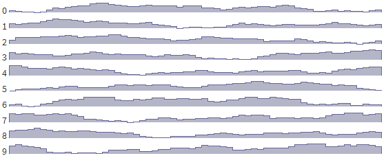
What if I used them as weights
[0.1, 0.1, 0.2, 0.3, 0.5, 1.0]? Low frequencies would be very light, and at high frequencies it would be much larger: All we have done here is a weighted sum of noise functions at different frequencies, and this took less than 15 lines of code. We can generate a wide range of different noise styles.
Summarize:
- Instead of selecting an array of random numbers, we select a single random number and use it to shift the sine wave left or right.
- You can create noise by taking a weighted sum of other noise functions having different frequencies.
- You can select noise characteristics by selecting weights for the weighted sum.
8. Rainbow generation
Now that we can generate noise by mixing noise together at different frequencies, let's look at the color of the noise again.
Let's go back to the Wikipedia page on noise colors . Note that the frequency spectrum is indicated there . He tells us about the amplitude of each frequency present in the noise. White noise - flat, pink and red are tilted down, blue and purple rise up.
The frequency spectrum is correlated with our arrays
frequenciesand amplitudesfrom the previous section.Previously, we used frequencies that are powers of two. Different types of color noise have much more frequencies, so we need a larger array. For this code, instead of powers of two (1, 2, 4, 8, 16, 32), I'm going to use all integer frequencies from 1 to 30. Instead of writing the amplitudes manually, I will write a function
amplitude(f)that returns the amplitude of any given frequency and creates an array from these data amplitudes. We can again use the functions
weighted_sumand noise, but now instead of a small set of frequencies we will have a longer array:frequencies = range(1, 31) # [1, 2, ..., 30]
def random_ift(rows, amplitude):
for i in range(rows):
random.seed(i)
amplitudes = [amplitude(f) for f in frequencies]
noises = [noise(f) for f in frequencies]
sum_of_noises = weighted_sum(amplitudes, noises)
print_chart(i, sum_of_noises)
random_ift(10, lambda f: 1)In this code, the function
amplitudedefines the form. If it always returns 1, then we get white noise. How to generate other colors of noise? I use the same random seed, but use a different amplitude function for it:8.1. Red noise
random_ift(5, lambda f: 1/f/f)8.2. Pink noise
random_ift(5, lambda f: 1/f)8.3. White noise
random_ift(5, lambda f: 1)8.4. Blue noise
random_ift(5, lambda f: f)8.5. Purple noise
random_ift(5, lambda f: f*f)8.6. Noise colors
So, this is pretty convenient. You can change the exponent of the amplitude function to obtain simple shapes.
- Red noise is f ^ -2
- Pink noise is f ^ -1
- White noise is f ^ 0
- Blue noise is f ^ + 1
- Purple noise is f ^ + 2
Try changing the exponent [in the original article] to see how the noise from sections 8.1-8.5 is generated from one basic function.
Summarize:
- Noise can be generated by a weighted sum of sinusoids with different frequencies.
- Different colors of noise have weights (amplitudes) corresponding to the function f ^ c.
- By changing the exponent, different colors of noise can be obtained from one set of random numbers.
9. Other forms of noise
To generate different colors of noise, we forced the amplitudes to follow simple power functions with different exponents. But we are not limited only to these forms. This is the simplest pattern that appears in straight lines on the logarithmic graph. Perhaps there are other sets of frequencies that create interesting patterns for our needs. You can use an array of amplitudes and adjust them as you wish instead of using a single function. It's worth exploring, but I haven't done it yet.
What we did in the previous section can be perceived as Fourier series . The main idea is that any continuous function can be represented as a weighted sum of sinusoids and cosines. The appearance of the final function changes depending on the selected weights.The Fourier transform connects the original function with its frequencies. Usually we start with the source data and get the frequencies / amplitudes from them. This can be seen in music players showing the “spectrum” of noise.
Direct direction allows you to analyze data and get frequencies; the reverse direction allows you to synthesize data from frequencies. In noise work, we usually do synthesis. In fact, we already did this. In the previous section, we selected frequencies and amplitudes and generated noise.
The Fourier transform has many uses.
On this pageThere is an explanation of how the Fourier transform works. The diagrams on this page are interactive - you can enter the strength of each frequency, and the page will show how they combine. By combining sinusoids, you can get many interesting shapes. For example, try typing Cycles input in the box
0 -1 0.5 -0.3 0.25 -0.2 0.16 -0.14and unchecking the Parts check box. True, it looks like a mountain? In the Appendix (Appendix) of this page there is a version showing how the sinusoids look in polar coordinates. For an example of using the Fourier transform to generate maps, see the technique of generating landscapes by frequency synthesis.Paul Bourke, who first generates two-dimensional white noise, then converts it to frequencies using the Fourier transform, then gives it the shape of pink noise, and then converts it back using the inverse Fourier transform.
My little experience in experimenting with 2D shows that everything in it is not as straightforward as in 1D. If you want to look at my unfinished experiments, scroll to the end of this page and move the sliders .
10. Other noise functions
In this article, we used sinusoids to generate noise. It is pretty simple. We take several functions and summarize them. Even if the original functions do not look noisy, the result looks good enough, especially considering that we wrote only 15 lines of code.
I have not studied in detail other noise functions, but I use them in my projects. I think many of them generate pink noise:
- I believe that in the midpoint displacement, a sawtooth signal is used instead of a sinusoid, and then higher and higher frequencies with more and lower amplitudes are summed. I think it turns pink noise. As a result, we see noticeable faces that arise either due to a sawtooth signal (not as smooth as sinusoids), or due to the use of only frequencies that are powers of two. I don’t know for sure.
- Diamond square — это вариация midpoint displacement, которая позволять скрыть грани, получаемые в midpoint displacement.
- Одна октава шума Перлина/симплекс-шума генерирует сглаженный шум с определённой частотой. Чтобы сделать шум розовым, обычно суммируются несколько октав шума Перлина.
- Мне кажется, что фрактальное броуновское движение (ФБД) тоже генерирует розовый шум суммированием нескольких функций шума.
- Алгоритм Восса-Маккартни выглядит похожим на midpoint displacement. Он суммирует несколько функций белого шума с разными частотами.
- Direct pink noise can be generated by calculating the inverse Fourier transform for the desired frequencies. This is exactly what the example in the previous section does. Paul Bourke describes it as Frequency Synthesis and demonstrates how it looks for 2D noise generating three-dimensional height maps.
Some information about the Voss-McCartney algorithm makes me think that summing noise at different frequencies is not quite pink noise, but close enough to it to generate maps. The joints received in midpoint displacement are most likely due to it, or maybe due to the interpolation function, I don’t know for sure.
I did not find many ways to generate blue noise.
- Для моего проекта генератора карт я использовал алгоритм Ллойда с диаграммами Вороного, чтобы сгенерировать нужный мне синий шум. У меня уже была библиотека, создающая диаграммы Вороного, поэтому было проще снова использовать её, чем реализовывать как отдельный этап.
- Ещё один способ генерирования синего шума — пятна Пуассона. Если в вашем проекте ещё не используется библиотека Вороного, то пятно Пуассона выглядит проще. См. также эту статью, описывающую использование пятна в играх.
- Рекурсивные плитки Вана тоже могут генерировать синий шум. Я пока ещё не изучал их, но надеюсь взяться за это в будущем.
- Может быть, получится также напрямую генерировать синий шум, вычисляя обратное преобразование Фурье из спектра частот синего шума, но я пока не пробовал.
I'm not even sure that I need the right blue noise for the cards, but this is described in the literature as blue noise. The blue noise that I generate using sine waves is similar to what I need, but the techniques listed above, it seems to me, should be better suited for games.
11. Additional reading
This article was originally notes for myself. When I published, I improved the diagrams and added a couple of interactive ones. I spent much less time on it than on my other articles, but I experimented with explaining some of the topics, hoping that this would allow me to cover more information.
I also have experiments with 2D that are not as polished as the data in this article. Including there is a 3D-visualization of a two-dimensional height map .
Other topics I didn’t go into much:
- The libnoise page has a fantastic explanation of noise and interpolation functions, including an explanation of why the interpolation function should have smooth derivatives
- В этом введении в шум Перлина объясняются теория, стоящая за шумом Перлина, и связанные с ним функции шума
- В ещё одном введении в шум Перлина также описывается теория
- В этом введении в двухмерное преобразование Фурье есть куча отличных изображений, которые помогут в интуитивном понимании пространства частот
- green_meklar на reddit рассказывает о способах комбинирования и искажения шума для генерирования ландшафтов
- В Math/StackExchange есть описания преобразования Фурье
- Как создавать одномерный и двухмерный шум
- Заметки Стефана Густавсона (Stefan Gustavson) о шуме Перлина, в том числе о том, как делать его бесшовным, и о том, почему иногда стоит предпочесть вместо него симплекс-шум
- Страница из книги, описывающей ФБД
- На этой и этой страницах объясняется принцип работы быстрого преобразования Фурье
- Использование нелинейных функций интерполяции
- Винеровский процесс
- Броуновский мост в Википедии
- Более математические заметки Джулиуса Смита (Julius Smith) о преобразовании Фурье, в особенности для работы с аудио
- Шум для процедурного генерирования планет
- Генерирование ландшафта с холмами вместо синусоид
- Генерирование шума в графическом процессоре
- Заметки Notch'а о генерировании ландшафта Minecraft — изначально он использовал и двухмерный шум Перлина для высот, и трёхмерный шум Перлина для порога плотности, но сейчас использует двухмерную карту высот, а пещеры генерирует с помощью червей Перлина
- Генерирование процедурного 3D-мира
- Creating seamless 2D noise functions - 4D noise is used instead of 2D noise mixing functions to create seamless 2D noise