VaR as a way of assessing risk. Historical method

In this article I want to introduce you to the popular financial risk assessment tool VaR ( ValueAtRisk ). In doing so, I will try to use a minimum of economic, mathematical and statistical terms.
The main ideas of VaR were developed and applied at JP Morgan in the 80s. VaR was widely used in 1993 when it was approved by the Group of Thirty (G-30) as part of the “best practices” for working with derivatives (derivative financial instruments). And later it became one of the bank’s risk indicators using the Basel II system (a set of international recommendations on banking regulation). The idea used in VaR can be traced back to the early work of Nobel laureate in economics Garia Markowitz in 1952.
Why do we need VaR?
VaR has many uses:
- banks determine current risk by department and bank in general;
- traders use VaR in trading strategies (for example, to determine when to exit a trade);
- private investors to choose less risky investments;
Management of risks
First, let's understand what risk management is and why it is needed.
“Risk management is the process of detecting, analyzing and making or mitigating uncertainties in investment decisions. In essence, risk management always happens when an investor or fund manager analyzes and tries to assess potential losses and then take (or not) the necessary measures, taking into account his investment objectives and risk tolerance. ”
→ Source
Why is risk management relevant? Daniel Kahneman in his book, Think Slowly ... Decide Quickly , argues that people do not like to lose more than they like to win. That is, if a person is offered to win $ 110 with 50% and lose $ 100 with 50%, then he will most likely refuse, although the potential gain is greater. The author calls this loss averse asymmetry.
Prediction of possible losses to which people are so sensitive, we will deal with. But before moving on to VaR, we need to talk about the concept of volatility , without which it is impossible to imagine risk management .
A bit about Volatility
First, consider two examples.
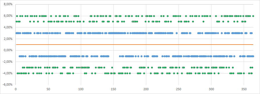
Example 1 - let stock A all day last year either grow by 3% or lose -1%. Moreover, these two events were independent and equally probable. If our investments are $ 100, then we can say with high probability that tomorrow the trend will continue and we will either receive $ 3, or lose -1 $ with the same probability. In other words, the probability of getting + 3 $ is 50% and the probability of losing -1 $ is also 50%. We can even say that the expected profit every day is $ 1 (3 $ * 50% -1 $ * 50%). But as we will see later, the expected profit is not what interests us in risk management. Losses are important to us, and with possible losses everything is clear here -with a 50% probability we can lose $ 1 .

Random income + 3% or -1%
Now let's look at example 2 . There is information about the daily earnings of stock B over the past year. Income Properties:
- took one of four values -4%, -3%, + 5%, + 6%;
- the probability of each of the four events is the same - 25%;
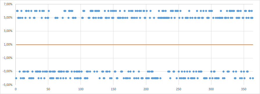
Random income -3%, -4%, 5% or 6%
I specifically selected the values so that the average value was +1% (- 4% * 25% -3% * 25% + 5% * 25% + 6% * 25%) as in the first example. That is, if we have stocks for $ 100, then the expected value tomorrow will also be $ 1 .
Comparison of Example 1 (-1%, + 3%) and Example 2 (-3%, -4%, 5%, 6%)
Although the expected values in the two cases are the same (+ 1%), the level of risk is different, because the size losses may be higher in the second case. This is volatility .
Volatility, volatility (English volatility) - a statistical financial indicator that characterizes the volatility of prices. It is the most important financial indicator and concept in financial risk management, where it is a measure of the risk of using a financial instrument for a given period of time.
Or in your own words, volatility is the power of spreading values. The larger the spread, the higher the volatility and the more difficult it is for us to make an assumption about the price in the future. The conclusion suggests itself, the higher the volatility, the higher the risk . It would seem that volatility is the indicator that we need.
But volatility has one significant drawback for risk management. It takes into account both the spread of profits and the spread of losses. For example, if the price of a share rises sharply, then volatility will increase. Although the risk, in terms of possible losses, will remain at the same level. This problem will be solved by VaR, but before moving on to VaR, let's deal with the problem of estimating losses.
Problem 1 . How to describe potential losses?
If in the first example the forecast of losses for tomorrow was -1% with a probability of 50% , then in the second example the situation is more complicated. We can say that:
- with a probability of 25% we will lose 3%;
- with a probability of 25% we will lose 4%;
- with a probability of 50% we will lose more than 3%;
All these statements are true, but we only have 4 possible outcomes . In real life, the number of outcomes can be much larger. Accordingly, the number of statements that we can make about the likelihood of risk will increase. And this complicates the reporting and analysis of information.
Problem 2. Extreme values.
Let's imagine that last year the stock took values from -5% to 5%, but in one day the loss was -10%. If we take the number of days in a year for 364 (for simplicity, forget about weekends and holidays), then the probability of a loss repeating at -10% is 1/364 = 0.274%. The probability of 0.274% is rather small, it is difficult to imagine, and someone may find it generally not significant for consideration. How to be in this case?
In both of these cases, VaR comes to our aid.
Var
VaR allows you to evaluate losses with a certain probability. And this can be done quite briefly, so that a person can relatively easily imagine the size of the risk. VaR answers the following question:
“ What is the maximum loss I can expect over a certain period of time with a given level of probability (confidence)”
For example, a $ 100 VaR with a threshold of 99% means:
- with a probability of 1% we can lose $ 100 or more during the day;
- with a probability of 99% we will not lose more than $ 100 during the day;
Both of these statements are equivalent.
VaR consists of three components:
- forecast level / threshold (usually 95% or 99%);
- forecast time interval (day, month or year);
- possible losses (amount of money (usually dollars) or interest);
The ability to choose a threshold (99% in our example) is a very convenient property for many investors. This property allows us to come closer to the answer to the question that worries many investors “ how much can we lose during the day (month) in the worst case? "
There are three methods for producing VaR: historical , covariance, and the Monte Carlo method .
In this article we will consider the historical method , since it requires the least knowledge in the field of statistics and, in my opinion, the most intuitive of the three.
VaR Counting Steps:
- Collect historical income data for a certain period (month, year);
- Sort data in ascending order;
- Choose the threshold with which we want to make a forecast and “cut off” the worst value knowing the threshold;
For clarity, let's go through this process of finding VaR for a real-life example. As an example, we look at Apple stock prices in 2015.
Steps:
1. Get data on stock returns as a percentage . You can download data, for example, from yahoo.finance.com. Yahoo provides opening, closing, and so on. We will consider closing prices (close *). Note that on yahoo, dates are sorted in descending order, so you can sort in ascending order. We will convert closing prices into profit as a percentage from the previous day. For example, if the price yesterday was $ 10, and today $ 15, then the percentage profit will be ($ 15 -10 $) / $ 10 = 50%;
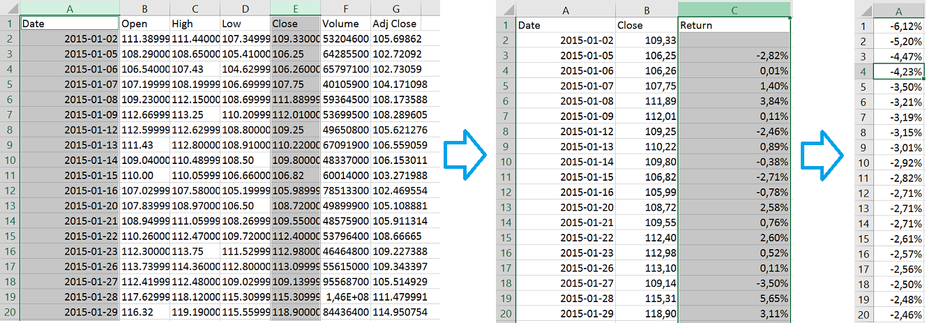 Converting data from Yahoo and sorting
2. Sort profits ascending (for clarity, I built a histogram);
3. Select the threshold with which we want to make a forecast and “cut off” the worst valueknowing the threshold. We have 252 working days. If we want to make an assessment covering 95% of cases, then we discard the worst 5%, the probability of which we consider low. 5% of 252 days is 13 days (round 12.6 to 13). If you look at the graph, you can see that the income of the 13th “worst day” was -2.71%. Now we can say that with a probability of 95% we will not lose more than 2.71%. If our investments are $ 100, then with a probability of 95% we will not lose more than $ 2.71. This does not mean that we cannot lose more than $ 2.71 , we are talking about a probability of 95%. If this is not enough, then you can increase the threshold, for example, to 99%;
* We select close price, not adj. close, since adj. close is inconsistent and can change over time. For example, if stock split occurs. Our goal is for the numbers to agree with those who will complete this example later.
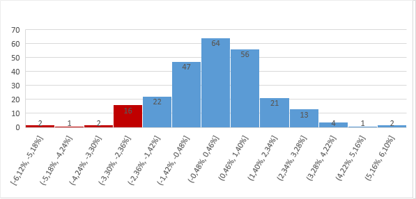 Concluding the example with Apple data, I’m giving you another interesting chart. On the chart, we see horizontal ranges of profits, and vertically - the number of days when profits fell into the corresponding interval. This graph is very similar to the normal distribution . This fact is useful to us in the next article where we will consider two other methods of calculating VaR.
Code example
    public Double calculateHistoricalVar(List prices, Double confidenceLevel, Double amount) {
        if (prices.isEmpty()) {
            return 0d;
        }
        List returns = getReturns(prices);
        Collections.sort(returns);
        double threshold = (returns.size() * (1 - confidenceLevel));
        int intPart = (int) threshold;
        Double decimalPart = threshold - intPart;
        Double rawVar = returns.get(intPart);
        Double interpolatedPart = decimalPart * (returns.get(intPart) - (returns.get(intPart + 1)));
        return rawVar + interpolatedPart;
    }
    private List getReturns(List prices) {
        List result = new ArrayList<>(prices.size());
        for (int i = 1; i < prices.size(); i++) {
            result.add(prices.get(i) / (prices.get(i - 1)) - 1);
        }
        return result;
    }
A little about the shortcomings of the historical method and VaR in general:
- We predict the future using historical data. This may be a fragile assumption. Since we make the assumption that events from the past will be repeated. You can try to deal with this using different time intervals to calculate VaR (year, month, day). We will talk about this below.
- VaR says nothing, about values outside the threshold, for example 95%. We can have two different stocks A and B with a VaR of $ 50 at a threshold of 95% and 100 observations. Let the 95 best observations of A and B be the same and equal from -50 $ to 45 $ in increments of 1 $. But the five worst profits are A = {-1000 $, -800 $, -700 $, -600 $, -500 $}, and B = {-100 $, -99 $, -98 $, -97 $, -96 $}. Obviously, the risk for B is higher. You can try to deal with this by increasing the threshold (up to 99%, 99.9%, 99.99%, etc.). There are also methods specifically designed to address these shortcomings, for example, Conditional VAR, which estimates losses if losses exceed VaR. But we will not consider them in this article.
Questions that may arise when working with VaR:
- How to choose a period?
- There is no definite answer to this, it all depends on your investment horizon. Banks usually consider VaR for days, pension funds, on the other hand, often consider VaR for months.
- What if 95% is not an integer item number?
- In our example, we used 252 days and a threshold of 95%. The element that we cut off is 252 * 0.05 = 12.6. In our example, we simply rounded and took the 13th element, but to be precise, our value should be somewhere in between. Unfortunately, in our example, the 12th and 13th elements are -2.71%. Therefore, let's imagine that the 12th element is -4%, and the 13th is -3%. Then VaR will be between -4% and -3%, closer to -3%. More precisely -3.6%. Here interpolation comes to our aid. The formula is as follows:
b + (ab) * k, where a is the lower value, b is the upper value and k is the fractional part (in our case 0.6)
It turns out -3% + (-4% + 3%) * 0.6 = -3.6%
Conclusion
The beauty of the VaR approach is that it works great for a set of several stocks or a combination of different securities. For example, VaR for a set of bonds and currencies gives us an estimate without much effort. And the use of other methods, such as the analysis of possible scenarios, is greatly complicated due to the correlation (connection) between securities.
→ Source