Why do we need the Ho-Kashyap algorithm?
Recently, a publication appeared on Habré about the Ho-Kashyap algorithm (Ho-Kashyap procedure, aka - the algorithm of the NSCE, the least standard error). It seemed to me not very clear and I decided to figure it out myself. It turned out that the topic is not very well understood on the Russian-speaking Internet, so I decided to write an article based on the results of searches.
Despite the boom in neural networks in machine learning, linear classification algorithms remain much simpler to use and interpret. But at the same time, sometimes I don’t feel like using any advanced methods, such as the support vector method or logistic regression, and there is a temptation to drive all the data into one large linear MNC regression, moreover, even MS Excel is able to build it perfectly.
The problem with this approach is that even if the input data is linearly separable, the resulting classifier may not separate them. For example, for a set of points![X = [(6, 9), (5, 7), (5, 9), (10, 1)]](https://tex.s2cms.ru/svg/%20X%20%3D%20%5B(6%2C%209)%2C%20(5%2C%207)%2C%20(5%2C%209)%2C%20(10%2C%201)%5D%20) ,
, ![y = [1, 1, -1, -1]](https://tex.s2cms.ru/svg/%20y%20%3D%20%5B1%2C%201%2C%20-1%2C%20-1%5D%20) we get the dividing line
we get the dividing line %20%3D%200%20) (the example is borrowed from (1)):
(the example is borrowed from (1)):
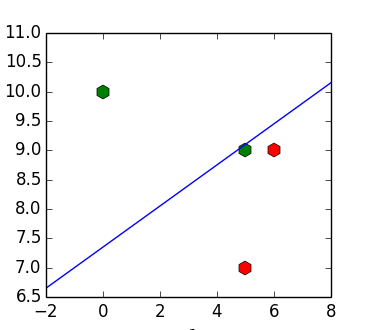
The question arises - is it possible to somehow get rid of this feature of behavior?
First, we formalize the subject of the article.
A matrix is given , each line of
  which corresponds to a characteristic description of the object
  (including a constant
  ) and the vector of class labels
  , where
  is the label of the object . We want to build a linear view classifier
 %20%3D%20y%20) .
.
The easiest way to do this is to construct an OLS regression for , that is, minimize the sum of the squared deviations
 %5E2%20) . Optimal weights can be found by the formula
. Optimal weights can be found by the formula  , where
  is the pseudoinverse matrix. Thus, a picture is obtained from the beginning of the article.
For the convenience of writing, we multiply each line of inequalityby element by element  and call the matrix obtained on the left side
  (here, it
  means row- wise multiplication). Then the condition for OLS regression is reduced to the form
  , and the minimization problem is minimized
 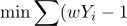%5E2%20) .
.
At this point, we can recall that the condition for separating classes isor %20%3D%201%20) , and since we want to separate classes, we must solve this problem.
, and since we want to separate classes, we must solve this problem.
We introduce a vector in which
  is responsible for the distance from the element to the dividing line (
  ). Since we want all elements to be classified correctly, we introduce a condition
  . Then the problem will be reduced to
 %5E2%20) and will be solved as
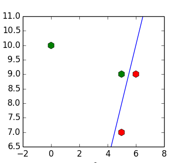
and will be solved as  . You can manually select such values that the resulting plane will separate our sample:
The Ho-Kashyap algorithm is designed to beautomatically selected . Algorithm scheme (  - step number,
 %7D%20) usually taken equal ):
usually taken equal ):
I want to calculate the indent vector in some way, sort of%7D%20%3D%20%5Cmax(Yw%5E%7B(k)%7D%2C%200)%20) , since this minimizes the loss function . Unfortunately, the condition does not allow us to do this, and instead it is proposed to take a step along the positive part of the gradient of the loss function
, since this minimizes the loss function . Unfortunately, the condition does not allow us to do this, and instead it is proposed to take a step along the positive part of the gradient of the loss function %7D%20%3D%20b%5E%7Bk%7D%20-%20Yw%5E%7B(k)%7D%20) :,
:, %7D%20%3D%20b%5E%7B(k)%7D%20-%20%5Cmu%20(e%5E%7B(k)%7D%20-%20%7Ce%5E%7Bk%7D%7C)%20) where
where  is the step of the gradient descent, decreasing in the course of solving the problem.
In the case of a linearly separable sample, the algorithm always converges and converges to the separating plane (if all elements of the gradient arenonnegative, then they are all zero).
If linearly inseparable sample loss function can be arbitrarily small, since it is sufficient to multiplyand  by a constant to change its value and, in principle, the algorithm may not converge. The search does not give any specific recommendations on this topic.
You may notice that if the object is classified correctly, then the error in the posed optimization problem (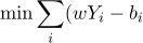%5E2%20) ), the error on it can be reduced to zero. If the object is classified incorrectly, then the minimum error on it is equal to the square of its indent from the dividing line (
), the error on it can be reduced to zero. If the object is classified incorrectly, then the minimum error on it is equal to the square of its indent from the dividing line ( %5E2%20) ). Then the loss function can be rewritten in the form:
). Then the loss function can be rewritten in the form:
%5E2%20-%202%5Cmax(0%2C%201%20-%20w%20Y_i)%20%20)
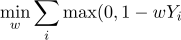
In turn, the linear SVM loss function has the form:
%20)
Thus, the problem solved by the Ho-Kashyap algorithm is an analogue of SVM with a quadratic loss function (it fines heavier for emissions far from the separating plane) and ignoring the width of the separating strip (i.e., looking for a non-plane located as far as possible from the nearest correctly classified elements, but any dividing plane).
We may recall that MNC regression is an analogue of Fisher's two-class linear discriminant (their solutions coincide up to a constant). The Ho-Kashpyap algorithm can also be applied to the case of classes - in this they become matrices of
  both
both  size
size  and,
and,  respectively, where
  is the dimension of the problem, and
  is the number of objects. In this case, the columns corresponding to the incorrect classes must have negative values.
parpalak for a convenient editor.
rocket3 for the original article.
Despite the boom in neural networks in machine learning, linear classification algorithms remain much simpler to use and interpret. But at the same time, sometimes I don’t feel like using any advanced methods, such as the support vector method or logistic regression, and there is a temptation to drive all the data into one large linear MNC regression, moreover, even MS Excel is able to build it perfectly.
The problem with this approach is that even if the input data is linearly separable, the resulting classifier may not separate them. For example, for a set of points
The question arises - is it possible to somehow get rid of this feature of behavior?
Linear classification problem
First, we formalize the subject of the article.
A matrix is given
>>> import numpy as np
>>> X = np.array([[6, 9, 1], [5, 7, 1], [5, 9, 1], [0, 10, 1]])
>>> y = np.array([[1], [1], [-1], [-1]])
The easiest way to do this is to construct an OLS regression for
>>> w = np.dot(np.linalg.pinv(X), y)
>>> w
array([[ 0.15328467],
       [-0.4379562 ],
       [ 3.2189781 ]])
>>> np.dot(X, w)
array([[ 0.19708029],
       [ 0.91970803],
       [ 0.04379562],
       [-1.16058394]])
Linear separability
For the convenience of writing, we multiply each line of inequality
>>> Y = y * X
>>> Y
array([[  6,   9,   1],
       [  5,   7,   1],
       [ -5,  -9,  -1],
       [  0, -10,  -1]])
At this point, we can recall that the condition for separating classes is
We introduce a vector
>>> b = np.ones([4, 1])
>>> b[3] = 10
>>> w = np.dot(np.linalg.pinv(Y), b)
>>> np.dot(Y, w)
array([[  0.8540146 ],
       [  0.98540146],
       [  0.81021898],
       [ 10.02919708]])
Ho Kashyap Algorithm
The Ho-Kashyap algorithm is designed to be
- Calculate the OLS regression coefficients (
).
- Calculate the indentation vector
.
- If the solution does not fit (
), then repeat step 1.
I want to calculate the indent vector in some way, sort of
>>> e = -np.inf * np.ones([4, 1])
>>> b = np.ones([4, 1])
>>> while np.any(e < 0):
...     w = np.dot(np.linalg.pinv(Y), b)
...     e = b - np.dot(Y, w)
...     b = b - e * (e < 0)
...
>>> b
array([[  1.],
       [  1.],
       [  1.],
       [ 12.]])
>>> w
array([[ 2.],
       [-1.],
       [-2.]])
In the case of a linearly separable sample, the algorithm always converges and converges to the separating plane (if all elements of the gradient are
If linearly inseparable sample loss function can be arbitrarily small, since it is sufficient to multiply
Connection of the Ho-Kashyap algorithm and linear SVM
You may notice that if the object is classified correctly, then the error in the posed optimization problem (
In turn, the linear SVM loss function has the form:
Thus, the problem solved by the Ho-Kashyap algorithm is an analogue of SVM with a quadratic loss function (it fines heavier for emissions far from the separating plane) and ignoring the width of the separating strip (i.e., looking for a non-plane located as far as possible from the nearest correctly classified elements, but any dividing plane).
Multidimensional case
We may recall that MNC regression is an analogue of Fisher's two-class linear discriminant (their solutions coincide up to a constant). The Ho-Kashpyap algorithm can also be applied to the case of
Acknowledgments
parpalak for a convenient editor.
rocket3 for the original article.
References
(1) http://www.csd.uwo.ca/~olga/Courses/CS434a_541a/Lecture10.pdf
(2) http://research.cs.tamu.edu/prism/lectures/pr/pr_l17.pdf
( 3) http://web.khu.ac.kr/~tskim/PatternClass Lec Note 07-1.pdf
(4) A.E. Lepsky, A.G. Bronevich Mathematical methods for pattern recognition. Lecture Course
(5) Tu J., González R. Principles of Pattern Recognition
(6) R. Duda, P. Hart Pattern Recognition and Scene Analysis