Reinforcement training for the smallest
This article discusses the principle of the machine learning method “Learning with reinforcement” using the example of a physical system. The optimal strategy search algorithm is implemented in Python code using the Q-Learning method .
Reinforced learning is a machine learning method in which a model is trained that does not have information about the system, but has the ability to perform any actions in it. Actions transfer the system to a new state and the model receives some reward from the system. Consider the operation of the method using the example shown in the video. The video description contains the code for Arduino , which is implemented in Python .
Using the reinforcement training method, it is necessary to teach the trolley to drive away from the wall to the maximum distance. The award is presented as the value of the change in the distance from the wall to the trolley during movement. The distance D from the wall is measured by a range finder. The movement in this example is possible only with a certain offset of the "drive", consisting of two arrows S1 and S2. Arrows are two servos with guides connected in the form of a “knee”. Each servo in this example can rotate 6 equal angles. The model has the ability to perform 4 actions, which are the control of two servos, action 0 and 1 rotate the first servo by a certain angle clockwise and counterclockwise, steps 2 and 3 rotate the second servo drive a certain angle clockwise and counterclockwise. Figure 1 shows a working prototype of a trolley.

Fig. 1. Trolley prototype for experiments with machine learning
In Figure 2, arrow S2 is highlighted in red, arrow S1 is highlighted in blue, and 2 servos are black.

Fig. 2. System engine The system
diagram is shown in Figure 3. The distance to the wall is indicated by D, the range finder is shown in yellow, the system drive is highlighted in red and black.

Fig. 3. System diagram The
range of possible positions for S1 and S2 is shown in Figure 4:

Fig. 4.a. Boom position range S1

Fig. 4.b. Boom position range S2
The actuator limit positions are shown in Figure 5:
With S1 = S2 = 5, the maximum distance from the ground.
With S1 = S2 = 0, the minimum range to the ground.

Fig. 5. Boundary positions of arrows S1 and S2
The “drive” has 4 degrees of freedom. An action changes the position of arrows S1 and S2 in space according to a certain principle. The types of actions are shown in Figure 6.
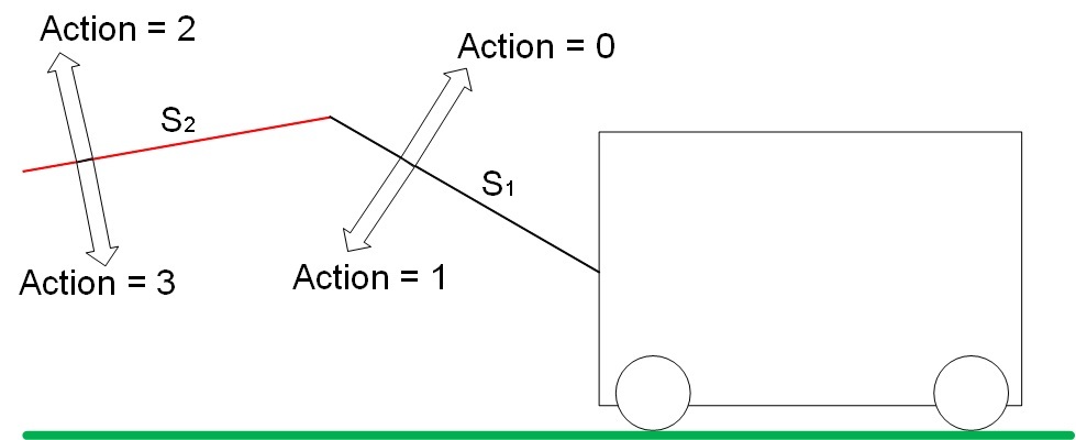
Fig. 6. Types of actions (Action) in the system.
Action 0 increases the value of S1. Step 1 reduces the value of S1.
Step 2 increases the value of S2. Step 3 decreases the S2 value.
In our problem, the trolley is driven in only 2 cases:
In position S1 = 0, S2 = 1, action 3 sets the trolley in motion from the wall, the system receives a positive reward equal to the change in the distance to the wall. In our example, the reward is 1.
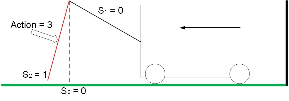
Fig. 7. Movement of the system with positive reward
In position S1 = 0, S2 = 0, action 2 drives the trolley to the wall, the system receives a negative reward equal to the change in the distance to the wall. In our example, the reward is -1.

Fig. 8. Movement of the system with a negative reward
In other conditions and any actions of the “drive”, the system will stand still and the reward will be 0.
It should be noted that the stable dynamic state of the system will be a sequence of actions 0-2-1-3 from the state S1 = S2 = 0, in which the trolley will move in a positive direction with a minimum number of actions taken. Raised the knee - straightened the knee - lowered the knee - bent the knee = the trolley moved forward, repeat. Thus, using the machine learning method, it is necessary to find such a state of the system, such a certain sequence of actions, the reward for which will not be received immediately (actions 0-2-1 - the reward for which is 0, but which are necessary to obtain 1 for the next action 3 )
The basis of the Q-Learning method is a matrix of system state weights. The matrix Q is a collection of all possible states of the system and the weights of the reaction of the system to various actions.
In this problem, possible combinations of system parameters 36 = 6 ^ 2. In each of the 36 states of the system, it is possible to perform 4 different actions (Action = 0,1,2,3).
Figure 9 shows the initial state of the matrix Q. The zero column contains the row index, the first row is the S1 value, the second is the S2 value, the last 4 columns are weights with actions equal to 0, 1, 2, and 3. Each row represents a unique state of the system.
When initializing the table, we equate all the values of the weights 10.
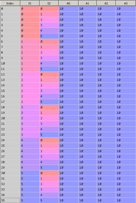
Fig. 9. Initialization of the matrix Q
After training the model (~ 15000 iterations), the matrix Q has the form shown in Figure 10.

Fig. 10. Matrix Q after 15,000 iterations of training.
Please note that actions with weights of 10 are not possible in the system, so the value of the weights has not changed. For example, in the extreme position with S1 = S2 = 0, actions 1 and 3 cannot be performed, since this is a limitation of the physical environment. These border actions are prohibited in our model, so the algorithm does not use 10k.
Consider the result of the algorithm:
...
Iteration: 14991, was: S1 = 0 S2 = 0, action = 0, now: S1 = 1 S2 = 0, prize: 0
Iteration: 14992, was: S1 = 1 S2 = 0, action = 2, now: S1 = 1 S2 = 1, prize: 0
Iteration: 14993, was: S1 = 1 S2 = 1, action = 1, now: S1 = 0 S2 = 1, prize: 0
Iteration: 14994, was: S1 = 0 S2 = 1, action = 3, now: S1 = 0 S2 = 0, prize: 1
Iteration: 14995, was: S1 = 0 S2 = 0, action = 0, now: S1 = 1 S2 = 0, prize: 0
Iteration: 14996, was: S1 = 1 S2 = 0, action = 2, now: S1 = 1 S2 = 1, prize: 0
Iteration: 14997, was: S1 = 1 S2 = 1, action = 1, now: S1 = 0 S2 = 1, prize: 0
Iteration: 14998, was: S1 = 0 S2 = 1, action = 3, now: S1 = 0 S2 = 0, prize: 1
Iteration: 14999, was : S1 = 0 S2 = 0, action = 0, now: S1 = 1 S2 = 0, prize: 0
Let's
take a closer look : Take iteration 14991 as the current state.
1. The current state of the system is S1 = S2 = 0, this line corresponds to a row with index 0. The highest value is 0.617 (ignore the values of 10, described above), it corresponds to Action = 0. Therefore, according to the matrix Q, when the state of the system is S1 = S2 = 0 we perform action 0. Action 0 increases the value of the angle of rotation of the servo drive S1 (S1 = 1).
2. The next state S1 = 1, S2 = 0 corresponds to the line with index 6. The maximum value of the weight corresponds to Action = 2. Perform action 2 - increase S2 (S2 = 1).
3. The next state S1 = 1, S2 = 1 corresponds to the line with index 7. The maximum weight value corresponds to Action = 1. Perform action 1 - decrease S1 (S1 = 0).
4. The next state S1 = 0, S2 = 1 corresponds to the line with index 1. The maximum value of the weight corresponds to Action = 3. Perform action 3 - decrease S2 (S2 = 0).
5. As a result, they returned to the state S1 = S2 = 0 and earned 1 point of reward.
Figure 11 shows the principle of choosing the optimal action.

Fig. 11.a. Matrix Q
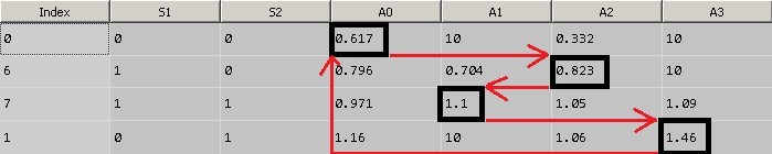
Fig. 11.b. Matrix Q
Let us consider the learning process in more detail.
Full code on GitHub .
Set the initial position of the knee to its highest position:
We initialize the matrix Q by filling in the initial value:
We calculate the epsilon parameter . This is the weight of the "randomness" of the algorithm in our calculation. The more iterations of training passed, the less random values of actions will be selected:
For the first iteration:
Save the current state:
Get the "best" value of the action:
Let's consider the function in more detail.
The getAction () function returns the value of the action that corresponds to the maximum weight in the current state of the system. The current state of the system in the Q matrix is taken and the action that corresponds to the maximum weight is selected. Note that this function implements a random action selection mechanism. As the number of iterations increases, the random choice of action decreases. This is done so that the algorithm does not focus on the first options found and can go on a different path, which may turn out to be better.
In the initial initial position of the arrows, only two actions 1 and 3 are possible. The algorithm chose action 1.
Next, we determine the row number in the Q matrix for the next state of the system, into which the system will go after performing the action that we received in the previous step.
In a real physical environment, after performing an action, we would get a reward if there was a movement, but since the movement of the cart is modeled, it is necessary to introduce auxiliary functions to emulate the reaction of the physical medium to actions. (setPhysicalState and getDeltaDistanceRolled ())
Let's execute the functions:
After completing the action, we need to update the coefficient of this action in the matrix Q for the corresponding state of the system. It is logical that if the action led to a positive reward, then the coefficient, in our algorithm, should decrease by a lower value than with a negative reward.
Now the most interesting thing is to look at the future to calculate the weight of the current step.
When determining the optimal action that needs to be performed in the current state, we select the largest weight in the matrix Q. Since we know the new state of the system that we switched to, we can find the maximum weight value from table Q for this state:
At the very beginning, it is 10. And we use the weight value of the action that has not yet been completed to calculate the current weight.
Those. we used the weight value of the next step to calculate the weight of the current step. The greater the weight of the next step, the less we will reduce the weight of the current (according to the formula), and the more the current step will be preferable the next time.
This simple trick gives good convergence results for the algorithm.
This algorithm can be expanded to a greater number of degrees of freedom of the system (s_features), and a larger number of values that the degree of freedom (s_states) takes, but within small limits. Fast enough, the Q matrix will take up all the RAM. Below is an example of the code for constructing a summary matrix of states and model weights. With the number of arrows s_features = 5 and the number of different positions of the arrow s_states = 10, the matrix Q has dimensions (100000, 9).
This simple method shows the “miracles” of machine learning, when a model without knowing anything about the environment learns and finds the optimal state in which the reward for actions is maximum, and the reward is not awarded immediately for any action, but for a sequence of actions.
Thanks for attention!
Reinforced learning is a machine learning method in which a model is trained that does not have information about the system, but has the ability to perform any actions in it. Actions transfer the system to a new state and the model receives some reward from the system. Consider the operation of the method using the example shown in the video. The video description contains the code for Arduino , which is implemented in Python .
Task
Using the reinforcement training method, it is necessary to teach the trolley to drive away from the wall to the maximum distance. The award is presented as the value of the change in the distance from the wall to the trolley during movement. The distance D from the wall is measured by a range finder. The movement in this example is possible only with a certain offset of the "drive", consisting of two arrows S1 and S2. Arrows are two servos with guides connected in the form of a “knee”. Each servo in this example can rotate 6 equal angles. The model has the ability to perform 4 actions, which are the control of two servos, action 0 and 1 rotate the first servo by a certain angle clockwise and counterclockwise, steps 2 and 3 rotate the second servo drive a certain angle clockwise and counterclockwise. Figure 1 shows a working prototype of a trolley.
Fig. 1. Trolley prototype for experiments with machine learning
In Figure 2, arrow S2 is highlighted in red, arrow S1 is highlighted in blue, and 2 servos are black.
Fig. 2. System engine The system
diagram is shown in Figure 3. The distance to the wall is indicated by D, the range finder is shown in yellow, the system drive is highlighted in red and black.
Fig. 3. System diagram The
range of possible positions for S1 and S2 is shown in Figure 4:
Fig. 4.a. Boom position range S1
Fig. 4.b. Boom position range S2
The actuator limit positions are shown in Figure 5:
With S1 = S2 = 5, the maximum distance from the ground.
With S1 = S2 = 0, the minimum range to the ground.
Fig. 5. Boundary positions of arrows S1 and S2
The “drive” has 4 degrees of freedom. An action changes the position of arrows S1 and S2 in space according to a certain principle. The types of actions are shown in Figure 6.
Fig. 6. Types of actions (Action) in the system.
Action 0 increases the value of S1. Step 1 reduces the value of S1.
Step 2 increases the value of S2. Step 3 decreases the S2 value.
Traffic
In our problem, the trolley is driven in only 2 cases:
In position S1 = 0, S2 = 1, action 3 sets the trolley in motion from the wall, the system receives a positive reward equal to the change in the distance to the wall. In our example, the reward is 1.
Fig. 7. Movement of the system with positive reward
In position S1 = 0, S2 = 0, action 2 drives the trolley to the wall, the system receives a negative reward equal to the change in the distance to the wall. In our example, the reward is -1.
Fig. 8. Movement of the system with a negative reward
In other conditions and any actions of the “drive”, the system will stand still and the reward will be 0.
It should be noted that the stable dynamic state of the system will be a sequence of actions 0-2-1-3 from the state S1 = S2 = 0, in which the trolley will move in a positive direction with a minimum number of actions taken. Raised the knee - straightened the knee - lowered the knee - bent the knee = the trolley moved forward, repeat. Thus, using the machine learning method, it is necessary to find such a state of the system, such a certain sequence of actions, the reward for which will not be received immediately (actions 0-2-1 - the reward for which is 0, but which are necessary to obtain 1 for the next action 3 )
Q-Learning Method
The basis of the Q-Learning method is a matrix of system state weights. The matrix Q is a collection of all possible states of the system and the weights of the reaction of the system to various actions.
In this problem, possible combinations of system parameters 36 = 6 ^ 2. In each of the 36 states of the system, it is possible to perform 4 different actions (Action = 0,1,2,3).
Figure 9 shows the initial state of the matrix Q. The zero column contains the row index, the first row is the S1 value, the second is the S2 value, the last 4 columns are weights with actions equal to 0, 1, 2, and 3. Each row represents a unique state of the system.
When initializing the table, we equate all the values of the weights 10.
Fig. 9. Initialization of the matrix Q
After training the model (~ 15000 iterations), the matrix Q has the form shown in Figure 10.
Fig. 10. Matrix Q after 15,000 iterations of training.
Please note that actions with weights of 10 are not possible in the system, so the value of the weights has not changed. For example, in the extreme position with S1 = S2 = 0, actions 1 and 3 cannot be performed, since this is a limitation of the physical environment. These border actions are prohibited in our model, so the algorithm does not use 10k.
Consider the result of the algorithm:
...
Iteration: 14991, was: S1 = 0 S2 = 0, action = 0, now: S1 = 1 S2 = 0, prize: 0
Iteration: 14992, was: S1 = 1 S2 = 0, action = 2, now: S1 = 1 S2 = 1, prize: 0
Iteration: 14993, was: S1 = 1 S2 = 1, action = 1, now: S1 = 0 S2 = 1, prize: 0
Iteration: 14994, was: S1 = 0 S2 = 1, action = 3, now: S1 = 0 S2 = 0, prize: 1
Iteration: 14995, was: S1 = 0 S2 = 0, action = 0, now: S1 = 1 S2 = 0, prize: 0
Iteration: 14996, was: S1 = 1 S2 = 0, action = 2, now: S1 = 1 S2 = 1, prize: 0
Iteration: 14997, was: S1 = 1 S2 = 1, action = 1, now: S1 = 0 S2 = 1, prize: 0
Iteration: 14998, was: S1 = 0 S2 = 1, action = 3, now: S1 = 0 S2 = 0, prize: 1
Iteration: 14999, was : S1 = 0 S2 = 0, action = 0, now: S1 = 1 S2 = 0, prize: 0
Let's
take a closer look : Take iteration 14991 as the current state.
1. The current state of the system is S1 = S2 = 0, this line corresponds to a row with index 0. The highest value is 0.617 (ignore the values of 10, described above), it corresponds to Action = 0. Therefore, according to the matrix Q, when the state of the system is S1 = S2 = 0 we perform action 0. Action 0 increases the value of the angle of rotation of the servo drive S1 (S1 = 1).
2. The next state S1 = 1, S2 = 0 corresponds to the line with index 6. The maximum value of the weight corresponds to Action = 2. Perform action 2 - increase S2 (S2 = 1).
3. The next state S1 = 1, S2 = 1 corresponds to the line with index 7. The maximum weight value corresponds to Action = 1. Perform action 1 - decrease S1 (S1 = 0).
4. The next state S1 = 0, S2 = 1 corresponds to the line with index 1. The maximum value of the weight corresponds to Action = 3. Perform action 3 - decrease S2 (S2 = 0).
5. As a result, they returned to the state S1 = S2 = 0 and earned 1 point of reward.
Figure 11 shows the principle of choosing the optimal action.
Fig. 11.a. Matrix Q
Fig. 11.b. Matrix Q
Let us consider the learning process in more detail.
Q-learning algorithm
minus = 0;
plus = 0;
initializeQ();
for t in range(1,15000):
    epsilon = math.exp(-float(t)/explorationConst);
    s01 = s1; s02 = s2
    current_action = getAction();
    setSPrime(current_action);
    setPhysicalState(current_action);
    r = getDeltaDistanceRolled();
    lookAheadValue = getLookAhead();
    sample = r + gamma*lookAheadValue;
    if t > 14900:
        print 'Time: %(0)d, was: %(1)d %(2)d, action: %(3)d, now: %(4)d %(5)d, prize: %(6)d ' % \
            {"0": t, "1": s01, "2": s02, "3": current_action, "4": s1, "5": s2, "6": r}
    Q.iloc[s, current_action] = Q.iloc[s, current_action] + alpha*(sample - Q.iloc[s, current_action] ) ;
    s = sPrime;
    if deltaDistance == 1:
        plus += 1;
    if deltaDistance == -1:
        minus += 1;
print( minus, plus )
Full code on GitHub .
Set the initial position of the knee to its highest position:
s1=s2=5.We initialize the matrix Q by filling in the initial value:
initializeQ();We calculate the epsilon parameter . This is the weight of the "randomness" of the algorithm in our calculation. The more iterations of training passed, the less random values of actions will be selected:
epsilon = math.exp(-float(t)/explorationConst)For the first iteration:
epsilon = 0.996672Save the current state:
s01 = s1; s02 = s2Get the "best" value of the action:
current_action = getAction();Let's consider the function in more detail.
The getAction () function returns the value of the action that corresponds to the maximum weight in the current state of the system. The current state of the system in the Q matrix is taken and the action that corresponds to the maximum weight is selected. Note that this function implements a random action selection mechanism. As the number of iterations increases, the random choice of action decreases. This is done so that the algorithm does not focus on the first options found and can go on a different path, which may turn out to be better.
In the initial initial position of the arrows, only two actions 1 and 3 are possible. The algorithm chose action 1.
Next, we determine the row number in the Q matrix for the next state of the system, into which the system will go after performing the action that we received in the previous step.
setSPrime(current_action);In a real physical environment, after performing an action, we would get a reward if there was a movement, but since the movement of the cart is modeled, it is necessary to introduce auxiliary functions to emulate the reaction of the physical medium to actions. (setPhysicalState and getDeltaDistanceRolled ())
Let's execute the functions:
setPhysicalState(current_action);r = getDeltaDistanceRolled();After completing the action, we need to update the coefficient of this action in the matrix Q for the corresponding state of the system. It is logical that if the action led to a positive reward, then the coefficient, in our algorithm, should decrease by a lower value than with a negative reward.
Now the most interesting thing is to look at the future to calculate the weight of the current step.
When determining the optimal action that needs to be performed in the current state, we select the largest weight in the matrix Q. Since we know the new state of the system that we switched to, we can find the maximum weight value from table Q for this state:
lookAheadValue = getLookAhead();At the very beginning, it is 10. And we use the weight value of the action that has not yet been completed to calculate the current weight.
sample = r + gamma*lookAheadValue;
sample = 7.5
Q.iloc[s, current_action] = Q.iloc[s, current_action] + alpha*(sample - Q.iloc[s, current_action] ) ;
Q.iloc[s, current_action] = 9.75
Those. we used the weight value of the next step to calculate the weight of the current step. The greater the weight of the next step, the less we will reduce the weight of the current (according to the formula), and the more the current step will be preferable the next time.
This simple trick gives good convergence results for the algorithm.
Algorithm Scaling
This algorithm can be expanded to a greater number of degrees of freedom of the system (s_features), and a larger number of values that the degree of freedom (s_states) takes, but within small limits. Fast enough, the Q matrix will take up all the RAM. Below is an example of the code for constructing a summary matrix of states and model weights. With the number of arrows s_features = 5 and the number of different positions of the arrow s_states = 10, the matrix Q has dimensions (100000, 9).
Increasing degrees of freedom of the system
import numpy as np
s_features = 5
s_states = 10
numActions = 4
data = np.empty((s_states**s_features, s_features + numActions), dtype='int')
for h in range(0, s_features):
    k = 0
    N = s_states**(s_features-1-1*h)
    for q in range(0, s_states**h):
        for i in range(0, s_states):
            for j in range(0, N):
                data[k, h] = i
                k += 1
for i in range(s_states**s_features):
        for j in range(numActions):
            data[i,j+s_features] = 10.0;
data.shape
# (100000L, 9L)
Conclusion
This simple method shows the “miracles” of machine learning, when a model without knowing anything about the environment learns and finds the optimal state in which the reward for actions is maximum, and the reward is not awarded immediately for any action, but for a sequence of actions.
Thanks for attention!