State machines in the SimInTech dynamic simulation environment

Introduction

SimInTech is a medium for creating mathematical models of any systems, the equation of dynamics of which can be represented as input-output relations (DataFlow representation). To implement the state machine approach in the SimInTech environment, there was a block of conditional execution of a submodel, which provided a stop and start of the simulation according to a condition coming from outside. This approach provides the ability to divide the general model into states and at each moment of time only calculate those submodels whose execution conditions are set to true. However, such an implementation of the automatic approach is not very convenient, from the point of view of clarity, and required additional adjustment of the system parameters.

Currently, all the necessary settings are implemented in a special library of blocks, which provides the creation of system models in the form of finite state machines (State Flow view) and can be used to create control models.

This article shows an example of using elements of the finite state machine library to create a control system.

Formulation of the problem

To demonstrate the simulation using finite state machines, a boiler control model is used. If the temperature is lower than the set one, the controller ensures that the heater is turned on for a period of no more than 20 seconds, with a shutter speed between turns 40, as well as an indication of its status by turning the indicator light on and off.

When the heater is on, the heating power is constant and heats 1 liter of water at 1 degree per second.
With the heater turned off, the losses are constant and such that they cool 1 liter of water by 0.1 degrees per second.
The amount of water is 25 liters.

The algorithm of the automatic temperature control operates as follows:

As input actions to the controller are set:
1) The setpoint (setpoint) of the temperature to be ensured.
2) The current temperature value received from the temperature sensor.

Description of the model in terms of finite state machines

The operation of the state machines of the heater controller can be described as follows: The
machine has two states on and off.
At the initial moment of time, the active state is off.

The state is off.
There is no heat.
The indicator blinks green at a frequency of 5 seconds.
The transition between the states: from the off state to the on state is carried out if two conditions coincide: the controller is in the off state for more than 40 seconds and the temperature from the sensor is lower than the set point.

Status
On Heating is in progress.
The red heating indicator blinks at a frequency of 1 second.
The transition from the on state to the off state is carried out in two cases:
1) Heating was carried out for 20 seconds.
2) The temperature from the sensor has reached the set point.

The finite state machine diagram implementing this algorithm is shown in Figure 1:


Figure 1. The finite state machine operation diagram

Implementation of the state machine operation in SimInTech

Creating an object model

The heater model is created using standard SimInTech modeling tools and is a submodel at the input of which the heater is turned on (0 - off, 1 - on), the water temperature is calculated at the output.

Place the “Submodel” block from the “Substructures” tab on the circuit and assemble the model as shown in Figure 2.


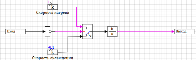
Figure 2. Heater model

A logical variable is applied to the unit input - a sign of heater operation, 1 - heater is on, 0 - heater is off. This variable is inverted and fed to the key "A3". Depending on this variable, the key transmits to the output the values ​​obtained from blocks of the "Constant" type: 1 - heating, or -0.1 - cooling. The output of the key block “A3” is integrated by a standard integrator. Thus, temperature values ​​are formed. The parameters of the integrator block are shown in Figure 3.


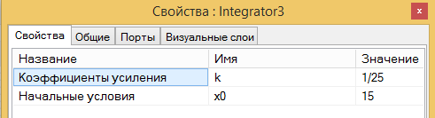
Figure 3. Integrator parameters The

initial temperature is 15, the gain is 1/25 (25 liters are heated at a given speed).
To check the operation of the heater model at the input, we supply a value from the Meander block, output the output to a graph along with the input. The model diagram is shown in Figure 4.


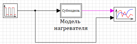
Figure 4. The general scheme for checking the heater model.

The simulation result is shown in Figure 5. During periods of time when the meander value is 1 (simulating the heater turned on), the model accumulates the temperature at the heating rate due to the integrator. In periods when the meander values ​​are 0 (simulation of the heater turned off), the temperature decreases with the cooling rate.


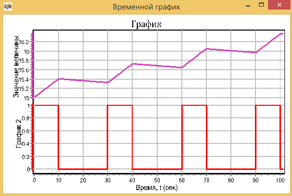
Figure 5. Schedule of the heater model.

Thus, we made sure that the created model can be used to check the operation of the heater controller.

Creation of a heater control unit based on state machines

To create the controller, we use the “State machine state map” block on the “State machines” tab. See Figure 6:


Figure 6. “Finite state machines” tab, “State machine state carat”

block Place the block on the diagram together with the “Heater model” block created earlier. Since this block is based on the standard SimInTech submodel, you can work with it the same way as with the submodel: add inputs and outputs, add signals, add properties, declare and use internal variables, link it to the signal database.
Go inside the “State machine state map” block by double-clicking on it. The only difference from the standard submodel is the presence of an additional block on the internal circuit, “State selection block” in the left corner of the circuit (see Fig. 7)

Before proceeding to the creation of a state map, we will prepare in this block the inputs and outputs necessary for the controller to communicate with the heater model.

The set and actual temperatures will be used as an input, the state of the heater on-off and the indication of the bulb will be calculated as the output.

Place two Entry Port blocks and two Exit Port blocks from the Substructures tab on the diagram and change their names as shown in Figure 7:


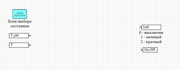
Figure 7. The state machine map prepared for data exchange

At this stage, you can exit the block by double-clicking on the empty meta of the circuit, and at the upper level, the block “State machine of the state machine” will display blocks — input and output ports — for connecting to the general circuit. Connect the circuit and sign the blocks as shown in Figure 8:


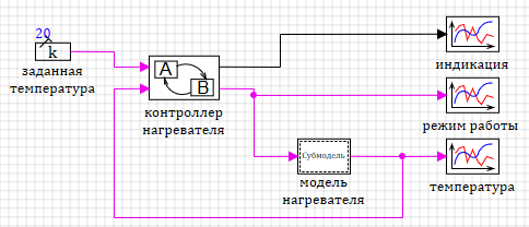
Figure 8. Block “Machine state”

Put two blocks “Machine state” on the circuit inside the block “Heater controller”. One of the blocks will simulate the state off, the other on. Sign the blocks accordingly, as shown in Figure 9.


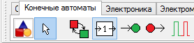
Figure 9. Block “Machine Status”

Place two “Machine Status” blocks on the circuit inside the “Heater Controller” block. One of the blocks will simulate the state off, the other on. Sign the blocks accordingly, as shown in Figure 10.


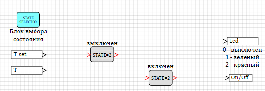
Figure 10. Controller layout with two added states.

For the state map to work correctly, you must specify the initial state of the system. In our case, the initial state of the machine will be off. Select the block with a click and right-click. In the drop-down menu, select "Properties". A window for editing properties will appear, in which you need to select yes in the only property “Default” (see Fig. 11):


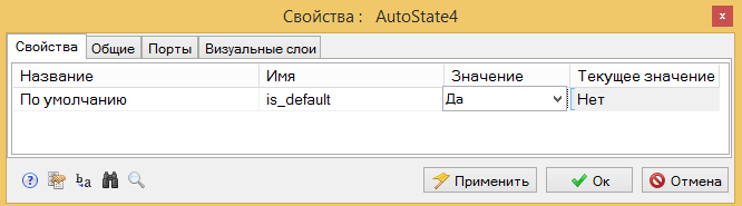
Figure 11. Setting the properties of the first active state in the map

Before proceeding to the creation of the logic of the operation of automata and transitions between states, we add the logic block “More” to the circuit and compare the set temperature with the temperature obtained from the model. Thus, we get a new logical variable that takes the value 1 when the temperature is less than the setpoint, and 0 when the temperature is greater than or equal to the setpoint.

Add the “More” block and connect the circuit as shown in Figure 12:

Figure 12: Comparison of the set and measured temperature

Note that SimInTech does not allow the output of the “More” block to be connected to the input of the “Machine state” block, since in the first case the line provides transmission values ​​between the blocks, and in the second - the transition from state to state.

Creating state logic

Double-click on the off state block to make a transition to the internal structure of the block. The initial internal structure of the block is shown in Figure 13:


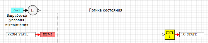
Figure 13. Internal structure of the “Machine Status” block The

internal structure contains, by default, the “Development of execution conditions” block at the top of the scheme. This block receives a command to activate the state from the top-level structure (“State block”), the user does not need to change this block.
In addition, the block contains two blocks of "input-output" of a special type:
1) "FROM_STATE" - entry into the state;
2) "TO_STATE" - exit from the state;
These ports correspond to the input and output to the block in the upper level circuit. These blocks are located on the tabs “Finite state machines”: blocks “Status input” and “Status output”, respectively.
The circuit of the automatic machines provides one state for the state to be turned on (if two conditions coincide: it is turned off for 40 seconds and the temperature is less than the set value), but returning to the state is possible according to two conditions: either the heater works for 20 seconds or the set temperature is reached. Add the “Status Input” block from the “Finite state machines” tab to the diagram (see Figure 14):


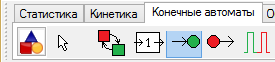
Figure 14. The “Finite state machines” tab of the “State input” block

Since we need the value of external comparison of the set temperature with the measured temperature to calculate the condition for exiting the state, add the “Input port” block from the “Substructures” tab to the diagram (see Fig. 15)


Figure 15. “Substructures” tab of the “Input port” block

To get the results of calculations performed in this state, add the “Output port” block from the “Substructures” tab to the diagram (see Figure 16):


Figure 16. “Substructures” tab of the “Output port” block

Change the name of the “Input” port to “Cold” "- there will be a comparison variable constant temperature with a given, and the name of the port "Exit" on the «On / Off» - here we read a sign on and off the heater.
The general scheme prepared for creating the state logic is presented in Figure 17.


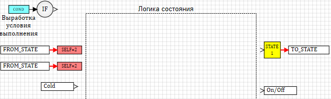
Figure 17. The “Machine state” block prepared for creating the logic

In the off state, the machine should be on for 40 seconds. If after a given period of time the water temperature is less than the set value (Cold input = 1), it is necessary to switch to the on state. To form a delay, we use the block “State exposure block”. (see Fig. 18):


Figure 18. “Finite state machines” tab “Exposure state

block ” This block, connected to the output of the “Execution condition” block, starts the timer and generates an end time signal at a specified interval. Place the block on the field and set the shutter speed to 40.

The shutter end signal is combined with an external signal (Сold) through the logical block “and”. If they coincide (the shutdown time has ended and the temperature is below the setpoint), then we form a command to exit the state and at the same time send a signal to turn on the heater to turn on. The general logic of operation is shown in Figure 19.


Figure 19 The logic of operation in the “off” state

When forming the output from the status block, it must be taken into account that the block in the active state constantly calculates and generates the value of the output signals (in our case, it is the On / Off output). When the state is completed and exited, the last calculated value remains on the line. In our case, at the exit from the state, a value of 1 will be generated and it will remain until the state is again active.

After the creation of the model of work in the off state is completed, we will go up one level by double-clicking on an empty place in the circuit (see Fig. 20).


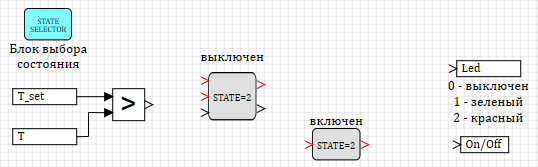
Figure 20. The state map diagram after editing the “off”

block . The appearance of the state block turned off has changed in the diagram. After adding the input and output ports inside the status block, three input ports and two output ports appeared on the block outside. The color of standard ports for signal transmission is black, the color of ports for connecting state transition lines is red. The user cannot connect data lines to status ports and, conversely, state transition lines to data ports.

We proceed to the formation of the logic of work in the on state.

Go inside the block by double-clicking on the image. For this block there will be two conditions for exiting the state. By default, there is one “Status Output” in the block. Place the second block “Status output” on the status diagram (see Fig. 21):


Figure 21. The “State machines” block of the “State output” block

In order to create an exit condition, you need to transfer the temperature comparison value to the block. To do this, we will add the “Port of exit” block from the “Substructures” tab to the diagram (see Fig. 15).

To control the operation for 20 seconds, put the block “Exposure state” on the circuit (see Fig. 17), and set it as the parameter “Time to transition to another state” - 20.

The general structure of the logic of the block will look like shown on figure 22:


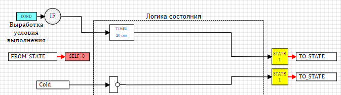
Figure 22. The structure of the work in the “on” state

When the switch to the on state, the work delay timer starts, after the time has passed, the transition to the first output is performed.

At the same time, the value obtained from the input with the data is analyzed. On this port we will submit the result of comparing the set temperature with the measured one. If the result is 1 (true), the temperature in the boiler is lower than the set value and you need to continue heating. If the value is 0 (false), then you need to complete the heating. The “operator NOT” block provides inversion of the input and generation of a command to switch from the state turned on by the second output (see. Fig. 22).

Let's move on to the top level of this scheme. Two additional ports appeared on the machine status block. And now the block contains:
• one input port to switch to the state (red);
• one input port for data (black);
• two output ports for transition from state (red).
Connect the ports as shown in Figure 23:


Figure 23. The logic of the operation of the state machine assembly

Thus, we have prepared a control model based on state machines for testing. At this stage, we connected the indicator output to the enable port in order to eliminate an error associated with an unconnected input port.
The indicator port at this stage displays the status (on / off). We will do modeling of intervals and indicator colors later.

Call the settings by calculating by clicking on the button “Calculation parameters” (see. Fig. 24):


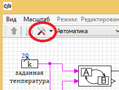
Figure 24. Button “Calculation parameters”

On the tab “Calculation parameters” set “Final calculation time” 700 seconds. (see Fig. 25)


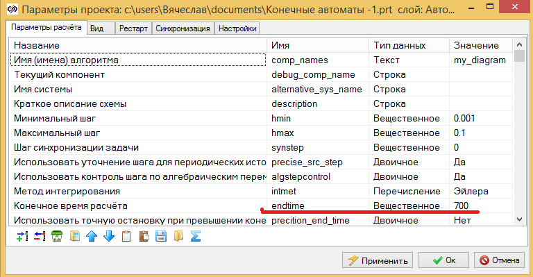
Figure 25. Calculation parameters

On the “Synchronization” tab, check the box “Synchronize with real time” and “Acceleration coefficient” - 100 (see Fig. 26).


Figure 26. Calculation parameters. Synchronization

By setting the synchronization mode, we can observe the switching between the states of the model directly on the diagram. Otherwise, the calculation is too fast and the state switching can only be tracked by graphs.
Run the model for calculation by pressing the start button (see. Fig. 27).


Figure 27. Launching the calculation of the model

If you assembled everything according to the instructions, then you received a model of a water heater controlled by a system based on the logic of finite state machines. In the controller diagram, during the simulation, one can observe the switching from state to state; the active state at the time of simulation is displayed in green (see Fig. 28).


Figure 28. Scheme of finished machines in simulation mode. The simulation

results are presented in Figures 29 (heater operation mode) and 30 (boiler temperature). The graph of the operating mode shows that at the initial time, the machine is in the off state (see Fig. 29).


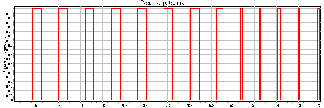
Figure 29. Heater operation mode


Figure 30. Heater temperature

The temperature graph (Fig. 30) shows that at the initial moment the temperature is 15 degrees and decreases with the cooling rate. After being in the off state, a transition to the on state occurs for 40 seconds (see Fig. 29). In this state, heating occurs at the speed specified in the heater model (see Fig. 30). After working out for 10 seconds, a transition to the off state occurs (see Fig. 29). These cycles are repeated until the temperature reaches the setpoint of 20 degrees. After that, the on cycle is shortened, since the transition from the on state to the off state is carried out upon reaching the temperature setting. This can be seen in the “Operating mode” graph after 500 seconds of calculation (see Fig. 29).

Thus, we were convinced that the control model based on the logic of finite state machines works and maintains a given temperature in the heater.

Please note that the signal on and off (On / Off) we form in the block is turned off, since this state is active by default and its outputs at the start are defined. When we exit this state, we change the signal value by 1 (see Figure 18) and it remains in the on state (1) all the time, while the state is not active. Since there are only two states in this finite state machine, we can apply this signal to the output from the state map. With any active state, the signal value will be determined and correct. If we have more than two states, then the exit from the “State Map” submodel must be determined or calculated in each block of states, otherwise it is possible to use variables that are not defined due to an inactive state.

The next part of the article will be:
- Demonstration of other data exchange capabilities in a finite state machine circuit.
- The process of creating a nested state machine for modeling the operation of the indicator. Part 2 here ....
- The process of obtaining C code from the created control system model.

A trial version of SimInTech can be downloaded from the developer's site. Here ...