Building Perfect Optics at Zemax
The construction of ideal optics in Zemax
Introduction
More and more modern automation systems are equipped with optical devices for solving problems of positioning, recognition, observation, etc. The construction of ideal optical systems using the Zemax calculation program can be useful to non-professionals, for example, for a better understanding of the theory and features of optical devices and performing approximate calculations of optical systems. In this work, methods of constructing ideal optics in Zemax environment are considered, examples of calculating the autofocus range of the camera, constructing the equivalent circuit of the MGT 2.5x17.5 monocular, the camera lens of the SUNNY P13N05B smartphone Huawei P7 and replacing the ideal optical elements with real ones are given.
Perfect optics
The image in ideal optics, in which there is no distortion, is built according to the laws of paraxial optics. The term paraxial means "near the axis." Paraxial optics are well described by linear expressions, which at small angles are replaced by linear equations. In the paraxial region, any real system behaves as ideal.
Calculation of ideal lenses in Zemax is carried out under the assumption that the lenses have paraxial properties not only close to the axis, but also on the entire working surface, which acts as an ideal thin lens with a single refractive index of air.
It is advisable to use paraxial optics as a standard with which aberrations (distortions) of real optics are compared.
To transfer the results of calculations of paraxial optics to real systems should be used with caution, especially when building systems in which the properties near the optical axis and at a distance are significantly different.
A number of techniques have been developed to reduce aberrations and overall dimensions of lenses: the use of non-spherical surfaces, composite lenses, heterogeneous optical materials, etc. But how would a real lens (Pettsval, Gauss, Barlow, ...) not be arranged, its characteristics can only approach characteristics of an ideal lens.
Image building with a collecting lens
Consider the case when rays from each point of the plane of the object diverge in all directions as from point sources. From the extreme point of object A, as shown in Fig. 1. only those rays that are focused by the lens will fall into the corresponding point B on the image plane. The number of rays of an object falling into the image plane is proportional to the diameter of the lens. The more rays from an object that fall into the image plane, the higher the brightness of the image.
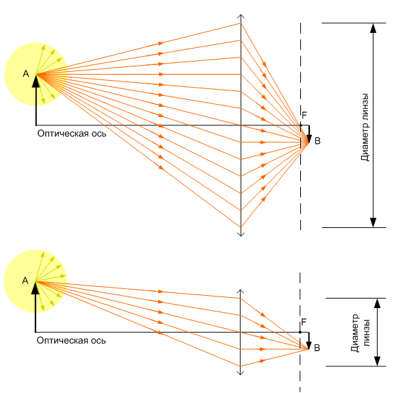
Fig. 1. Conjugate points. The path of the rays from the point of the object to the corresponding point of the
image on the plane of the photodetector.
To minimize the calculation of finding the image, only a few rays are considered, for example, as in Fig. 2: a beam coming from an object along the optical axis; a beam passing through the center of the lens and a beam parallel to the optical axis refracted by the lens and passing through the main focus of the lens (point F on the optical axis).
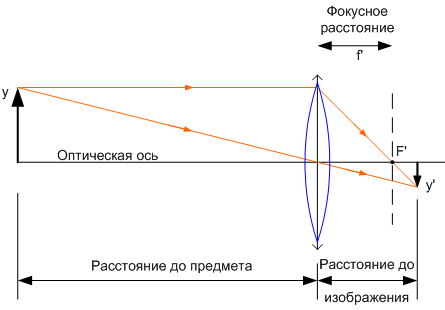
Fig. 2. Minimum construction for finding the distance to the image plane, image size and magnification of the lens. For paraxial optics, the longitudinal magnification (associated with distances) is equal to the square of the linear magnification (perpendicular to the axis), and the angular magnification is inversely proportional to linear.
The relationship of the distances to the subject and the image. Depth of field
The construction of the relationship between the focus area of the lens and the depth of field in the space of objects [1] is shown in Fig. 3. When the distance to the subject is equal to infinity, the plane of the focused image passes through the main focus (the shift of the image plane relative to the focus is zero). The minimum depth of field in the space of objects is achieved with the maximum distance of the image plane (in the focus area) relative to the main focus.
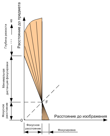
Fig. 3. The relationship between the focus area of the lens and the depth of field in the space of objects.
Functions of the Zemax design environment
The functions of the Zemax environment that are most often used in the design of optical systems are assigned to individual buttons on the main menu. The purpose of these buttons is shown in Fig. 4.

Fig. 4. The interface of the Zemax program.
Types of surfaces of elements of optical systems, radii of surfaces, distances between elements and other parameters are entered in the editor table, in which each line contains the parameters of one element. The relationship between the table parameters and the elements of the optical scheme is shown in the example of Fig. 5.
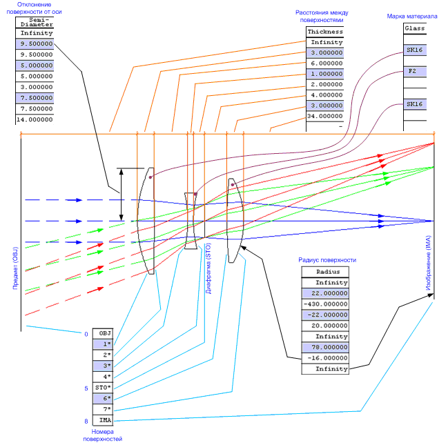
Fig. 5. The relationship of the optical scheme with the table parameters.
An ideal lens in Zemax
To model a lens with a paraxial surface in Zemax, you need to set the focal length and, if necessary, enable the calculation of the difference in optical paths passing through the lens (set the OPD mode status to 1 in the corresponding row of the editor table). By default, OPD calculation is not performed (OPD status is zero [2]).
We build in Zemax an ideal lens, for example, with an entrance pupil diameter of 10 mm and a focal length of 15 mm, collecting parallel rays of a distant object at one point.
1. Open a new table: menu> button
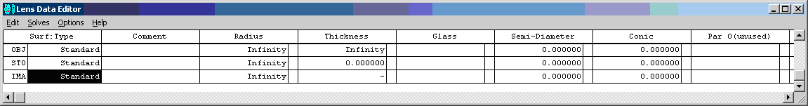
Fig. 6. The initial state of the table of the optical scheme of the Zemax editor. The rows of the table (NN 0; 1 and 2) contain the parameters of the subject OBJ, the aperture diaphragm STO and the IMA image.
2. Add the surface between the aperture and the image: select the last line the line IMA> menu Lens Data Editor> Edit> Insert Surface
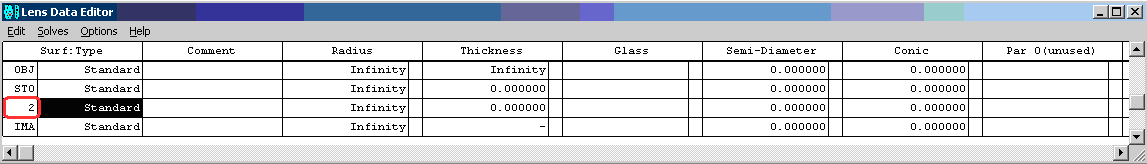
Fig. 7. Added standard N2 surface.
3. Select the “Paraxial” type of surface: line N2> column Surf: Type> property window - Properties> Surface Type> Paraxial
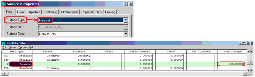
Fig. 8.N2 surface changed to a perfect (Paraxial) lens with a focal length of 100 mm. The distance between the lens and the image is zero. The distance between the lens and the STO aperture is also zero.
4. Change the focal length from 100 (default) to 15 mm in the column of the Focal Length table
5. Set the distance of 15 mm from the lens to the image in the Thickness column
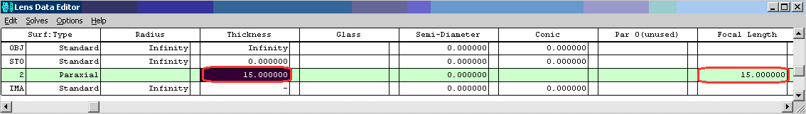
Fig. 9. The focal length of the lens is changed to 15 mm. The distance between the lens and the image is increased to 15 mm.
6. Set the entrance pupil diameter to 10 mm: Main menu> button> Aperture tab> Aperture Value> 10
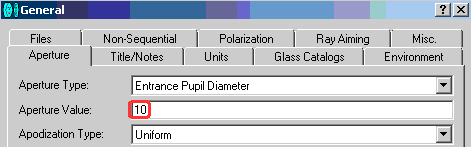
Fig. 10. The diameter of the input aperture of the optical circuit is set: 10 mm.
7. Build the optical scheme: Main menu> button
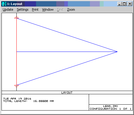
Fig. eleven.Optical design in the Layout window. The coordinates of the aperture and lens are the same (the distance between them is zero) The coordinates of the “mouse” in the diagram (on the scale of the optical diagram) are displayed in the title of the figure.
8. The Layout diagram does not show the rays to the left of the ideal lens (highlighted in red) coming from an object located at an infinite distance, which is indicated as Infinity in the Thickness column of the zero row of the OBJ table. To show part of these rays at the entrance of the lens, we introduce a surface at a distance of, for example, 7 mm in front of the STO aperture diaphragm.
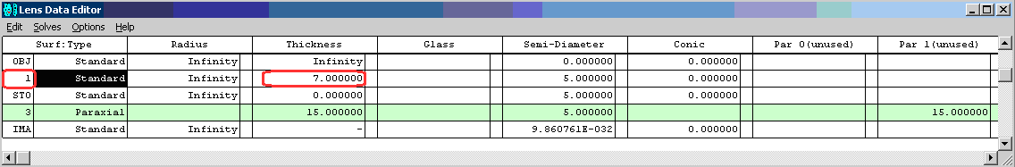
Fig. 12. Added surface in front of the STO aperture diaphragm.
9. Add surface 1 to the displayed part of the optical scheme and increase the number of rays to 7 for clarity: the picture menu Layout> Setting> First Surface = 1> Number of Rays = 7.
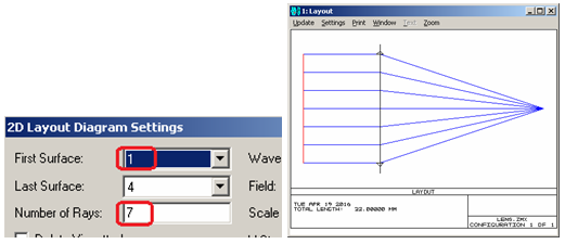
Fig. 13. The rays are shown at a distance of 7mm to the diaphragm. The number of rays has been increased from 3 to 7.
10. Make the first surface invisible: row N1 of the table> column Surf: Type> properties window - Properties> Draw tab>
11. Update the Layout window of the optical scheme through the main menu button or by double-clicking in the area of the circuit window.
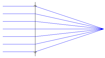
Fig. 14. The first surface of the optical circuit is made invisible.
In the Layout window, you can track changes in the table parameters of the optical system and the parameters of the main menu shown in Fig. 4 and Fig. 5.
Model of the composite lens of the smartphone’s camera
To build the ideal model, we take the composite lens of the SUNNY P13N05B camera of the Huawei P7 smartphone (Fig. 15). The lens of the smartphone consists of five plastic elements. An example of a composite lens is shown in Fig. 16.
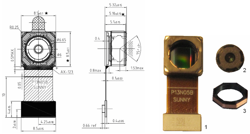
Fig. 15. Dimensions [3] and photographs of the SUNNY P13N05B camera with a 13 MP 13 SONY IMX214 photodiode array. 1. - camera module with a photodiode array; 2- camera lens; 3 - AF drive coil - moving the lens relative to the sensor matrix.
The P13N05B has the following features.
• Lens size: 1/3 ”
• Photodiode array size: 6.1 mm (H) × 4.5 mm (V)
• Diagonal of the active zone of the matrix: 5.9 mm
• Lens composition: 5 plastic elements (see. Fig. 16)
• Focal length: 3.79 mm
• Aperture number (f / #): 2
• Field of view: 75 ° ± 3 °
• Depth of field: 7 cm to ∞
• AF drive range: ≥ 0.24mm
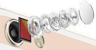
Fig. 16. An example of a composite lens. The lens of the iPhone 6 smartphone.
The optical scheme of the ideal camera lens (see Fig. 17) is specified in the Lens Data Editor table and in the key windows of the Zemax: main menu. The function selected from the list of functions of the selected cell in the Thickness column of the table automatically sets the best distance between the lens and the image. To build the best image of an object removed at an infinite distance, the plane of the photodetector must pass through the main focus point 3.79 mm away from the lens.
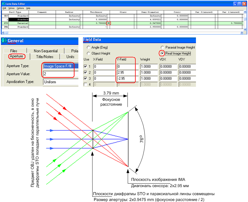
Fig. 17.Optical design of a paraxial lens of a photo lens. Item removed at infinite distance.
Approaching an object to the lens by 10 mm while maintaining a viewing angle of 76 ° / 2 in the Field Data window (Fig. 18) increased the distance between the lens and the image to 6.10 mm. Therefore, the change in autofocus when approaching an object from infinity to 10 mm is 2.31 mm (as 6.10 mm - 3.79 mm).
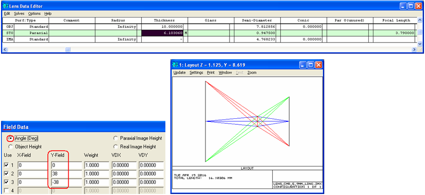
Fig. 18. The construction of rays from an object located 10 mm from the paraxial lens of the camera and finding the position of autofocus.
The specification of the camera P13N05B indicates that the depth of field in the space of objects lies in the range from 7 cm to ∞ (infinity). Set the item at a minimum distance of 70 mm from the lens aperture. Zemax sets the distance between the lens and the image plane to 4 mm (see the highlighted cell in the table in Fig. 19). Thus, to build a high-quality image of an object located in the zone from 7 cm to ∞, it is necessary to change the distance between the lens and the photosensor from 4 to 3.79 mm. The required change of 0.21 mm is covered by the range of the camera autofocus drive 0.24 mm.
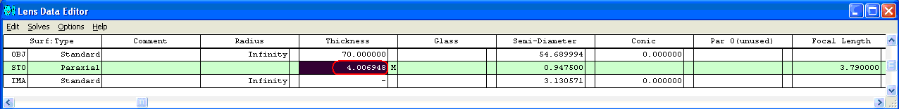
Fig. 19. The distance to the image is 4 mm and the distance to the object is 70 mm. The focal length of the lens is 3.79 mm.
The dependence of the focus range on the focal length of the lens
The focus area depends not only on the distance to the subject, but also on the main focus of the lens (lens). In Fig. 20 shows the geometry of finding the focus areas for lenses with the main focus F1 = 7.5 mm and F2 = 19 mm and the position of the subject in the range AB = 35 ... 52 mm. To adjust the sharpness with the F1 lens, it is necessary to change the distance between the main focus of the lens and the image plane in the range of 0.8 mm, while for the lens with F2 this range has grown to 12 mm.
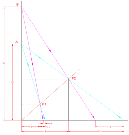
Fig. 20. An example of constructing focus areas for lenses with different focal lengths F1 and F2.
Perfect telescopes
The comparative dimensions of the Kepler and Galileo telescopes for the same magnification of F1 / F2 are shown in Fig. 21. Kepler's telescope with collecting lenses gives an inverted image. The more compact Galileo telescope includes a diffuser lens and gives a direct image.
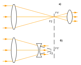
Fig. 21. Scheme of the Kepler (a) and Galileo (b) telescopes at the same magnification of F2 / F1.
The miniature monocular MGT 2.5x17.5 USSR, LZOS (Lytkarino Optical Glass Plant) was assembled according to the Galileo scheme (Fig. 22). It has the following characteristics.
• Magnification: 2.5 times (times)
• Lens diameter: 17.5 mm
• Field of view angle: 13.5 degrees
• Resolution: 15 angles. sec.
• Eyepiece focusing limit: -5 ... + 5 diopters
• Overall dimensions: 22 x 38 mm
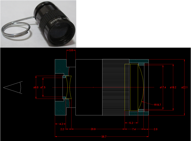
Fig. 22. View and approximate dimensions of the miniature monocular MGT 2.5x17.5. The subject is on the right.
The equivalent ideal optical design of the MGT 2.5x17.5 monocular in ZEMAX is shown in Fig. 23. The circuit consists of a collecting and scattering lens with the main foci of 37.5 mm and -15 mm, respectively, having a ratio of 2.5 times. The diameter of the collecting lens is 2x8.75 mm.
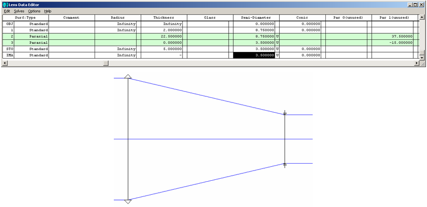
Fig. 23. Tabular data and the ideal optical design of the MGT monocular 2.5x17.5. Parallel rays come from an object removed at an infinite distance.
The option of replacing a paraxial lens with a real one
We replace the first paraxial lens (diameter: 17.5 mm; focal length: 37.5 mm) of the monocular with an achromatic lens from the Edmund Optics catalog [4]. To minimize the selection of lenses, we establish the following conditions: category - Achromatic Lenses; diameter - 18 mm; effective focal length EFL 30-39.99 mm; the wavelength range is 425 - 675 nm.
The lens closest to the required parameters: 18mm Dia. x 35mm FL, VIS 0 ° Coated, Achromatic Lens, Stock No. # 47-706 (catalog number).
To build an achromatic lens in Zemax, we take from the specification the parameters listed in Table 1. The parameters can also be found on the lens drawing PDF drawing of the Edmund Optics website [4] or in Fig. 24.
Table 1. Parameters of the composite achromatic lens Edmund # 47-706
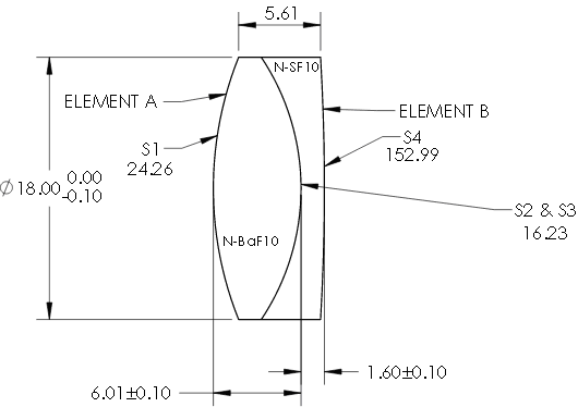
Fig. 24. Drawing achromatic lens Edmund # 47-706.
Replacing the parameters of the first lens of an ideal telescope (row N2 of the table in Fig. 23) with Edmund # 47-706 lens gives the option shown in Fig. 25.
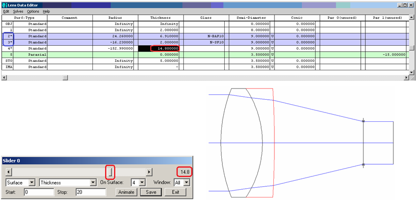
Fig. 25. Option optics telescope with a real achromatic lens. The distance between the lenses highlighted in the table in red was found by manually shifting the Slider engine.
The distance between the lenses (highlighted in red in the table in Fig. 25) was changed manually by the Slider until the rays at the output of the second (ideal lens) were set parallel to the main axis (in this position the focal lengths of the telescope lenses are at one point). The action of the slider in real time is displayed by the displacement of the elements of the optical scheme and the change of the ray paths on the optical diagram of the Layout window. The slider can be opened through the main menu Zemax> Tools> Miscellaneous> Slider.
If we put an additional paraxial collecting lens at the telescope’s output (element N6 in the table and the red plane in the optical diagram of Fig. 26), we can see the distortions introduced by the real lens (see part of the Zemax diagrams in Fig. 26).

Fig. 26. Optical design and distortion diagrams introduced by a real lens.
Literature
1. Optics Realm site. Video tutorials on designing in Zemax and optics theory. www.opticsrealm.com
2. Zemax Help> Optical Design Program User's Guide .pdf
3. H&L ELECTRICAL MANUFACTORY LIMITED hnl.en.e-cantonfair.com/products/sunny-brand-p13n05b-imx214-sony-sensor-13-0m -pixel-mipi-csi-1080p-sunny-cmos-camera-module-552104.html
4. Edmund Optics. www.edmundoptics.com/optics/optical-lenses
5. Dr. Bob Davidov. Computer control technologies in technical systems portalnp.ru/author/bobdavidov .
Introduction
More and more modern automation systems are equipped with optical devices for solving problems of positioning, recognition, observation, etc. The construction of ideal optical systems using the Zemax calculation program can be useful to non-professionals, for example, for a better understanding of the theory and features of optical devices and performing approximate calculations of optical systems. In this work, methods of constructing ideal optics in Zemax environment are considered, examples of calculating the autofocus range of the camera, constructing the equivalent circuit of the MGT 2.5x17.5 monocular, the camera lens of the SUNNY P13N05B smartphone Huawei P7 and replacing the ideal optical elements with real ones are given.
Perfect optics
The image in ideal optics, in which there is no distortion, is built according to the laws of paraxial optics. The term paraxial means "near the axis." Paraxial optics are well described by linear expressions, which at small angles are replaced by linear equations. In the paraxial region, any real system behaves as ideal.
Calculation of ideal lenses in Zemax is carried out under the assumption that the lenses have paraxial properties not only close to the axis, but also on the entire working surface, which acts as an ideal thin lens with a single refractive index of air.
It is advisable to use paraxial optics as a standard with which aberrations (distortions) of real optics are compared.
To transfer the results of calculations of paraxial optics to real systems should be used with caution, especially when building systems in which the properties near the optical axis and at a distance are significantly different.
A number of techniques have been developed to reduce aberrations and overall dimensions of lenses: the use of non-spherical surfaces, composite lenses, heterogeneous optical materials, etc. But how would a real lens (Pettsval, Gauss, Barlow, ...) not be arranged, its characteristics can only approach characteristics of an ideal lens.
Image building with a collecting lens
Consider the case when rays from each point of the plane of the object diverge in all directions as from point sources. From the extreme point of object A, as shown in Fig. 1. only those rays that are focused by the lens will fall into the corresponding point B on the image plane. The number of rays of an object falling into the image plane is proportional to the diameter of the lens. The more rays from an object that fall into the image plane, the higher the brightness of the image.
Fig. 1. Conjugate points. The path of the rays from the point of the object to the corresponding point of the
image on the plane of the photodetector.
To minimize the calculation of finding the image, only a few rays are considered, for example, as in Fig. 2: a beam coming from an object along the optical axis; a beam passing through the center of the lens and a beam parallel to the optical axis refracted by the lens and passing through the main focus of the lens (point F on the optical axis).
Fig. 2. Minimum construction for finding the distance to the image plane, image size and magnification of the lens. For paraxial optics, the longitudinal magnification (associated with distances) is equal to the square of the linear magnification (perpendicular to the axis), and the angular magnification is inversely proportional to linear.
The relationship of the distances to the subject and the image. Depth of field
The construction of the relationship between the focus area of the lens and the depth of field in the space of objects [1] is shown in Fig. 3. When the distance to the subject is equal to infinity, the plane of the focused image passes through the main focus (the shift of the image plane relative to the focus is zero). The minimum depth of field in the space of objects is achieved with the maximum distance of the image plane (in the focus area) relative to the main focus.
Fig. 3. The relationship between the focus area of the lens and the depth of field in the space of objects.
Functions of the Zemax design environment
The functions of the Zemax environment that are most often used in the design of optical systems are assigned to individual buttons on the main menu. The purpose of these buttons is shown in Fig. 4.
Fig. 4. The interface of the Zemax program.
Types of surfaces of elements of optical systems, radii of surfaces, distances between elements and other parameters are entered in the editor table, in which each line contains the parameters of one element. The relationship between the table parameters and the elements of the optical scheme is shown in the example of Fig. 5.
Fig. 5. The relationship of the optical scheme with the table parameters.
An ideal lens in Zemax
To model a lens with a paraxial surface in Zemax, you need to set the focal length and, if necessary, enable the calculation of the difference in optical paths passing through the lens (set the OPD mode status to 1 in the corresponding row of the editor table). By default, OPD calculation is not performed (OPD status is zero [2]).
We build in Zemax an ideal lens, for example, with an entrance pupil diameter of 10 mm and a focal length of 15 mm, collecting parallel rays of a distant object at one point.
1. Open a new table: menu> button
Fig. 6. The initial state of the table of the optical scheme of the Zemax editor. The rows of the table (NN 0; 1 and 2) contain the parameters of the subject OBJ, the aperture diaphragm STO and the IMA image.
2. Add the surface between the aperture and the image: select the last line the line IMA> menu Lens Data Editor> Edit> Insert Surface
Fig. 7. Added standard N2 surface.
3. Select the “Paraxial” type of surface: line N2> column Surf: Type> property window - Properties> Surface Type> Paraxial
Fig. 8.N2 surface changed to a perfect (Paraxial) lens with a focal length of 100 mm. The distance between the lens and the image is zero. The distance between the lens and the STO aperture is also zero.
4. Change the focal length from 100 (default) to 15 mm in the column of the Focal Length table
5. Set the distance of 15 mm from the lens to the image in the Thickness column
Fig. 9. The focal length of the lens is changed to 15 mm. The distance between the lens and the image is increased to 15 mm.
6. Set the entrance pupil diameter to 10 mm: Main menu> button> Aperture tab> Aperture Value> 10
Fig. 10. The diameter of the input aperture of the optical circuit is set: 10 mm.
7. Build the optical scheme: Main menu> button
Fig. eleven.Optical design in the Layout window. The coordinates of the aperture and lens are the same (the distance between them is zero) The coordinates of the “mouse” in the diagram (on the scale of the optical diagram) are displayed in the title of the figure.
8. The Layout diagram does not show the rays to the left of the ideal lens (highlighted in red) coming from an object located at an infinite distance, which is indicated as Infinity in the Thickness column of the zero row of the OBJ table. To show part of these rays at the entrance of the lens, we introduce a surface at a distance of, for example, 7 mm in front of the STO aperture diaphragm.
Fig. 12. Added surface in front of the STO aperture diaphragm.
9. Add surface 1 to the displayed part of the optical scheme and increase the number of rays to 7 for clarity: the picture menu Layout> Setting> First Surface = 1> Number of Rays = 7.
Fig. 13. The rays are shown at a distance of 7mm to the diaphragm. The number of rays has been increased from 3 to 7.
10. Make the first surface invisible: row N1 of the table> column Surf: Type> properties window - Properties> Draw tab>
11. Update the Layout window of the optical scheme through the main menu button or by double-clicking in the area of the circuit window.
Fig. 14. The first surface of the optical circuit is made invisible.
In the Layout window, you can track changes in the table parameters of the optical system and the parameters of the main menu shown in Fig. 4 and Fig. 5.
Model of the composite lens of the smartphone’s camera
To build the ideal model, we take the composite lens of the SUNNY P13N05B camera of the Huawei P7 smartphone (Fig. 15). The lens of the smartphone consists of five plastic elements. An example of a composite lens is shown in Fig. 16.
Fig. 15. Dimensions [3] and photographs of the SUNNY P13N05B camera with a 13 MP 13 SONY IMX214 photodiode array. 1. - camera module with a photodiode array; 2- camera lens; 3 - AF drive coil - moving the lens relative to the sensor matrix.
The P13N05B has the following features.
• Lens size: 1/3 ”
• Photodiode array size: 6.1 mm (H) × 4.5 mm (V)
• Diagonal of the active zone of the matrix: 5.9 mm
• Lens composition: 5 plastic elements (see. Fig. 16)
• Focal length: 3.79 mm
• Aperture number (f / #): 2
• Field of view: 75 ° ± 3 °
• Depth of field: 7 cm to ∞
• AF drive range: ≥ 0.24mm
Fig. 16. An example of a composite lens. The lens of the iPhone 6 smartphone.
The optical scheme of the ideal camera lens (see Fig. 17) is specified in the Lens Data Editor table and in the key windows of the Zemax: main menu. The function selected from the list of functions of the selected cell in the Thickness column of the table automatically sets the best distance between the lens and the image. To build the best image of an object removed at an infinite distance, the plane of the photodetector must pass through the main focus point 3.79 mm away from the lens.
Fig. 17.Optical design of a paraxial lens of a photo lens. Item removed at infinite distance.
Approaching an object to the lens by 10 mm while maintaining a viewing angle of 76 ° / 2 in the Field Data window (Fig. 18) increased the distance between the lens and the image to 6.10 mm. Therefore, the change in autofocus when approaching an object from infinity to 10 mm is 2.31 mm (as 6.10 mm - 3.79 mm).
Fig. 18. The construction of rays from an object located 10 mm from the paraxial lens of the camera and finding the position of autofocus.
The specification of the camera P13N05B indicates that the depth of field in the space of objects lies in the range from 7 cm to ∞ (infinity). Set the item at a minimum distance of 70 mm from the lens aperture. Zemax sets the distance between the lens and the image plane to 4 mm (see the highlighted cell in the table in Fig. 19). Thus, to build a high-quality image of an object located in the zone from 7 cm to ∞, it is necessary to change the distance between the lens and the photosensor from 4 to 3.79 mm. The required change of 0.21 mm is covered by the range of the camera autofocus drive 0.24 mm.
Fig. 19. The distance to the image is 4 mm and the distance to the object is 70 mm. The focal length of the lens is 3.79 mm.
The dependence of the focus range on the focal length of the lens
The focus area depends not only on the distance to the subject, but also on the main focus of the lens (lens). In Fig. 20 shows the geometry of finding the focus areas for lenses with the main focus F1 = 7.5 mm and F2 = 19 mm and the position of the subject in the range AB = 35 ... 52 mm. To adjust the sharpness with the F1 lens, it is necessary to change the distance between the main focus of the lens and the image plane in the range of 0.8 mm, while for the lens with F2 this range has grown to 12 mm.
Fig. 20. An example of constructing focus areas for lenses with different focal lengths F1 and F2.
Perfect telescopes
The comparative dimensions of the Kepler and Galileo telescopes for the same magnification of F1 / F2 are shown in Fig. 21. Kepler's telescope with collecting lenses gives an inverted image. The more compact Galileo telescope includes a diffuser lens and gives a direct image.
Fig. 21. Scheme of the Kepler (a) and Galileo (b) telescopes at the same magnification of F2 / F1.
The miniature monocular MGT 2.5x17.5 USSR, LZOS (Lytkarino Optical Glass Plant) was assembled according to the Galileo scheme (Fig. 22). It has the following characteristics.
• Magnification: 2.5 times (times)
• Lens diameter: 17.5 mm
• Field of view angle: 13.5 degrees
• Resolution: 15 angles. sec.
• Eyepiece focusing limit: -5 ... + 5 diopters
• Overall dimensions: 22 x 38 mm
Fig. 22. View and approximate dimensions of the miniature monocular MGT 2.5x17.5. The subject is on the right.
The equivalent ideal optical design of the MGT 2.5x17.5 monocular in ZEMAX is shown in Fig. 23. The circuit consists of a collecting and scattering lens with the main foci of 37.5 mm and -15 mm, respectively, having a ratio of 2.5 times. The diameter of the collecting lens is 2x8.75 mm.
Fig. 23. Tabular data and the ideal optical design of the MGT monocular 2.5x17.5. Parallel rays come from an object removed at an infinite distance.
The option of replacing a paraxial lens with a real one
We replace the first paraxial lens (diameter: 17.5 mm; focal length: 37.5 mm) of the monocular with an achromatic lens from the Edmund Optics catalog [4]. To minimize the selection of lenses, we establish the following conditions: category - Achromatic Lenses; diameter - 18 mm; effective focal length EFL 30-39.99 mm; the wavelength range is 425 - 675 nm.
The lens closest to the required parameters: 18mm Dia. x 35mm FL, VIS 0 ° Coated, Achromatic Lens, Stock No. # 47-706 (catalog number).
To build an achromatic lens in Zemax, we take from the specification the parameters listed in Table 1. The parameters can also be found on the lens drawing PDF drawing of the Edmund Optics website [4] or in Fig. 24.
Table 1. Parameters of the composite achromatic lens Edmund # 47-706
| Parameter | Value | Note |
|---|---|---|
| Diameter | 18.0 mm | Diameter |
| Clear aperture ca | 17.0 mm | Diaphragm |
| Effective Focal Length | 35.0 mm | Effective focal length |
| Center Thickness CT 1 | 6.01 mm | The thickness of the 1st element along the axis |
| Center Thickness CT2 | 1.60 mm | The thickness of the 2nd element along the axis |
| Radius R1 (mm) | 24.26 mm | Radius of the first surface |
| Radius R2 (mm) | 16.23 mm | The radius of the second surface |
| Radius R3 (mm) | -152.99 mm | Third surface radius |
| Substrate | N-BAF10 / N-SF10 | Element Materials |
Fig. 24. Drawing achromatic lens Edmund # 47-706.
Replacing the parameters of the first lens of an ideal telescope (row N2 of the table in Fig. 23) with Edmund # 47-706 lens gives the option shown in Fig. 25.
Fig. 25. Option optics telescope with a real achromatic lens. The distance between the lenses highlighted in the table in red was found by manually shifting the Slider engine.
The distance between the lenses (highlighted in red in the table in Fig. 25) was changed manually by the Slider until the rays at the output of the second (ideal lens) were set parallel to the main axis (in this position the focal lengths of the telescope lenses are at one point). The action of the slider in real time is displayed by the displacement of the elements of the optical scheme and the change of the ray paths on the optical diagram of the Layout window. The slider can be opened through the main menu Zemax> Tools> Miscellaneous> Slider.
If we put an additional paraxial collecting lens at the telescope’s output (element N6 in the table and the red plane in the optical diagram of Fig. 26), we can see the distortions introduced by the real lens (see part of the Zemax diagrams in Fig. 26).
Fig. 26. Optical design and distortion diagrams introduced by a real lens.
Literature
1. Optics Realm site. Video tutorials on designing in Zemax and optics theory. www.opticsrealm.com
2. Zemax Help> Optical Design Program User's Guide .pdf
3. H&L ELECTRICAL MANUFACTORY LIMITED hnl.en.e-cantonfair.com/products/sunny-brand-p13n05b-imx214-sony-sensor-13-0m -pixel-mipi-csi-1080p-sunny-cmos-camera-module-552104.html
4. Edmund Optics. www.edmundoptics.com/optics/optical-lenses
5. Dr. Bob Davidov. Computer control technologies in technical systems portalnp.ru/author/bobdavidov .