Can all financial models be wrong: 7 sources of risk of loss / ITI Capital Blog

ITI_Capital April 16, 2016 at 10:18

Can all financial models be wrong: 7 sources of risk of loss

On Habré and in the analytical section of our site, we write a lot about financial market trends and strategies for behavior on it. Very often, financial models, one way or another, are built on speculative conclusions. And how much the model relies on such data depends on its suitability for use. This indicator can be calculated using the risk model.

Turing Finance website creator and NMRQL hedge fund analyst Stuart Reed has published an interesting article on the analysis of possible risks of using financial models. The material discusses several factors that influence the occurrence of risks - that is, the probability of financial losses when using the model. We bring to your attention the main points of this work.

False premises

At the heart of any financial model are some assumptions. Therefore, when building a model, it is important to avoid the assumptions that make the model unsuitable for solving the tasks. We must not forget the "Occam's razor", do not multiply entities unnecessarily. This rule is especially critical when mastering machine learning. In our case, this principle can be interpreted as follows: if there is a choice between two models with equal predictive accuracy, one that uses fewer parameters will be more effective.

This does not mean that "a simple model is better than a complex one." This is one of the dangerous misconceptions. The main condition is the equivalence of predictions. It's not about the simplicity of the model. Working with complex computing technologies in finance makes any model indigestible, inelegant, but at the same time more realistic.

There are three varieties of false premises. No one says that these assumptions, usually taken on faith, make the model completely useless. The point is that there is a risk of its inefficiency.

1. Linearity

Linearity is the assumption that the relationship between any two variables can be expressed through a straight line of the graph. This view is deeply embedded in financial analysis, since most of the correlations are linear ratios of two variables.

That is, many are initially convinced that the ratio should be linear, although in reality the correlation may be non-linear. Such models may work for small forecasts, but not cover all their diversity. An alternative is to assume non-linear behavior. In this case, the model may not cover the entire complexity and inconsistency of the described system and may suffer from a lack of accuracy.

In other words, if you specify non-linear relationships, any linear measurements will either not be able to identify relationships at all, or will overestimate their stability and strength. What is the problem here?

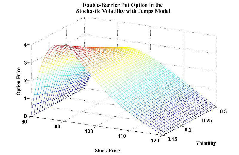
In portfolio management, the benefits of diversification are based on the use of a historical correlation matrix for selected assets. If the relationship between any two assets is non-linear (as happens with some derivatives), the correlation will overestimate or underestimate the gain. In this situation, the risks in the portfolio will become less or more than expected. If a company reserves capital for its needs and assumes a linear relationship between different risk factors, this will lead to an error in the amount of capital that needs to be reserved. Stress tests do not reflect the real risks of companies.

Plus, if during the development of the model classification is involved, where the relationship between the two data classes is non-linear, the algorithm may mistake them for one data class. A linear classifier can learn to handle non-linear data, for this you need to use the trick with kernels - the transition from scalar products to arbitrary kernels.

2. Stationarity

The meaning of the stationarity idea is that the trader creating the financial model is convinced that the variable or distribution from which it was extracted is constant in time. In many cases, stationarity is a perfectly reasonable assumption. For example, the “heavy” constant is unlikely to change significantly from day to day. That's why it is a constant. But for financial markets, which are adaptive systems, things are a bit confusing.

When assessing the risk of a model, it should be borne in mind that correlations, volatility, and risk factors may not be stationary. For each of them, the opposite belief leads to their own troubles.

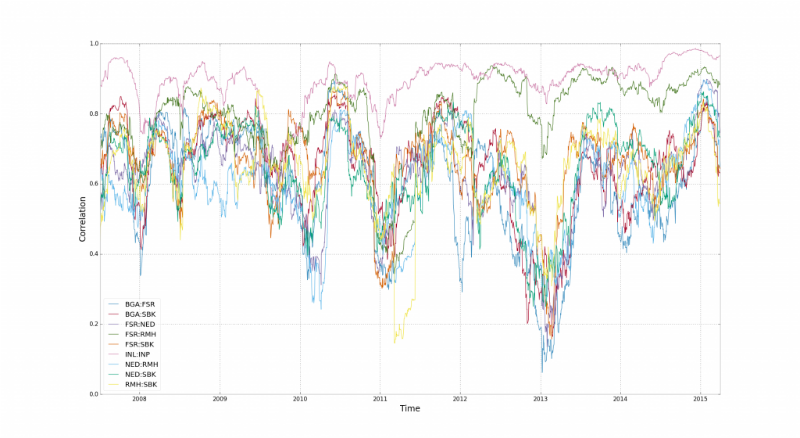
By correlation, it was written above. Here, the adoption of its stationarity distorts the risks of portfolio diversification. Correlations are unstable and “reset” during market reversals.

This chart shows the correlation behavior for 15 financial indices in South Africa. Here you can see the time intervals when the correlation breaks. According to Stuart Reed, it’s all about financial leverage , leverage - the shares of companies from different industries are “connected” by traders who trade them.

Volatility is also most often represented by a stationary variable. Especially if the stochastic approach is used in the price model for equity securities. Volatility is a criterion that determines how much income from securities varies over time. For example, for derivatives it is believed that the higher the volatility, the higher the price. Because there is a high probability that derivatives will lose their value. If the model underestimates volatility, most likely there is an underestimation of the value of derivatives.

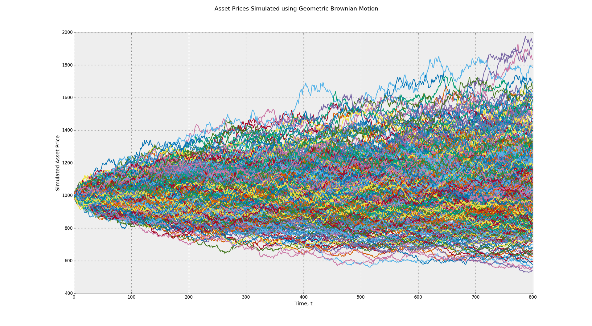
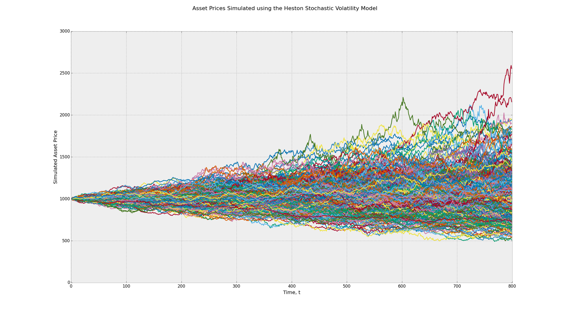
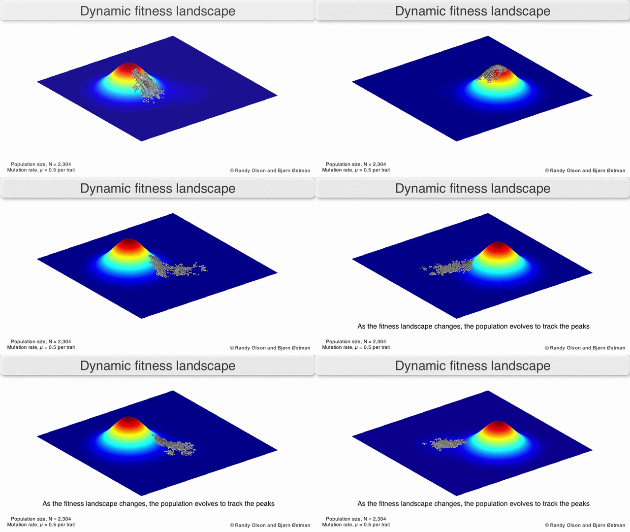
The stochastic process underlies the Black-Scholes model and works on the principle of Brownian motion. This model implies constant volatility over time. Feel the difference between the range of possible profits in this model and in the Heston model using the CIR indicator(Cox-Ingerosoll-Ross model) to determine random volatility. In the first graph, the range of potential final values lies between 500 and 2000. In the second case, it ranges from 500 to 2500. This is an example of the effect of volatility. In addition, many traders, when conducting a backtest of their strategy, by default accept the idea of the constancy of risk factors. In reality, factors such as momentum, the return of average values can have different effects when the state of the market changes seriously. The GIF below shows the dynamic distribution and how the genetic algorithm adapts to changes in the distribution over time. Such dynamic algorithms must be used when implementing risk management:

3. Normality

The assumption of normality means that our random variables follow the principle of normal (Gaussian) distribution. This is convenient for several reasons. The combination of any number of normal distributions eventually comes to a normal distribution itself. It is also easy to manage with the help of mathematical formulas, which means that mathematicians are able to create harmonious systems on its basis for solving complex problems.

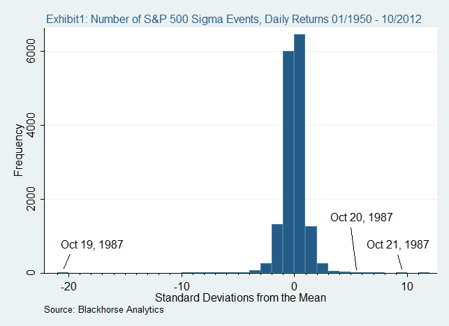
The catch is that many models, including the delta-normal approach, suggest that market portfolio returns also have a normal distribution. In the current market, profitability has its excesses and longer tails. This means that many companies underestimate the effect of the tail risk, which they reckon (or do not reckon) for the market crisis.

An example is the collapse of the market in 1987. On October 19 of that year, most stock markets around the world lost more than 20%. It is noteworthy that in a normal world where everything follows a normal distribution, this would be impossible.

Statistical distortion

Statistics are lying. If only does not satisfy anyone's interests. Ultimately, it all depends on how you calculate it. Below we discuss the most common causes of distortion in statistics that affect the result.

4. Sampling error

Often, sampling errors lead to a distortion of the statistical result. Simply put, the probability of a pattern represented in a sample depends directly on its probability in a real group. There are several methods for selecting a template. The most popular: random sampling, systematic sampling, stratified and cluster sampling.

In a simple random sample, each pattern has an equal chance of becoming part of the pattern. All this is suitable when the study area contains one class of patterns. Then simple sampling is fast and efficient. Another situation arises when several classes of patterns are available, the probability of each is spread across these classes. In this case, the sample will be unrepresentative, and the final result will be distorted.

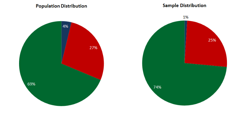
A stratified sample may be suitable for labeled data when a certain number of patterns are selected from each class according to its weight. For example, we have given patterns that belong to three classes - A. B, C. The distribution of patterns among them is 5%, 70% and 25%, respectively. That is, a sample of 100 patterns will contain 5 patterns of class A, 70 - B and 25 - C. This sample will be representative, but it can only be used for labeled data.

Multistage or cluster sampling allows a stratified approach to untagged data. At the first stage, the data is divided into classes using a cluster algorithm (k-means or ant algorithm). At the second stage, the selection is made in proportion to the weight and value of each class. Here the shortcomings of the previous methods are overcome, but the result begins to depend on the effectiveness of the cluster algorithm.

There is also a curse of dimension , which does not depend on the sampling technique used. It means that the number of patterns required for a representative sample increases exponentially with the attributes in these patterns. At a certain level, it becomes practically impossible to create a representative sample, which means to get an undistorted statistic result.

5. Fit Errors

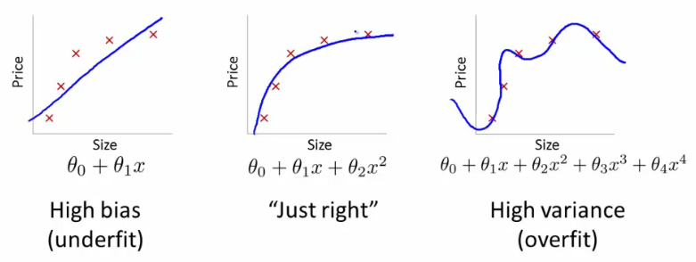
The so-called overfitting happens when the model describes the noise (randomness) in the data set, instead of establishing the basic statistical relationships. The performance within the sample will be fantastic, outside the sample - no. Such a model is usually said to have a low level of generalization. Over-fitting occurs where the model itself is too complex (or the learning strategy is too simple). Complexity and heaviness in this case are among the parameters that can be configured in the model.

In the quantum forums, you can find many descriptions of how re-fitting occurs. Stuart Reed is confident that quanta deliberately make this mistake in order to show their attitude to the use of complex Luddites. For example, deep neural networks in trading. Some go so far as to say that a simple linear regression will go over any complex model. These people do not take into account the effect of underfitting when the model is too simple to learn statistical wisdom.

But in any case, no matter what statistical errors the model sins, a lot depends on the training strategy. Many researchers use the cross-validation technique to avoid over -fitting.. She divides the data set into representative sections: training, testing and validation (confirmation of the result). Data is run through all three sections independently. If the model shows signs of over-fitting, its training is interrupted. The only drawback of this approach: for independent verification you need a large amount of data.

6. Durability

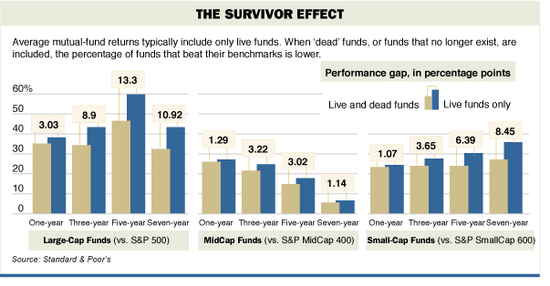
It will be a mistake to use for statistical analysis data that lives only on certain periods of time. A classic example of this is the use of hedge fund revenue data. Over the past 30 years, a bunch of funds have either skyrocketed or collapsed. If we use hedge fund data, then take only those that are currently working, Reid said. In this case, we exclude the risks that led to failure. This indicator is called the survivor effect. How it works is shown in the diagram.

7. Skipping variables

Another error manifests itself when one or more important casual variables are omitted . The model may incorrectly compensate for the missing variable by overestimating the value of other variables. This is especially critical if the included variables correlate with those that were not included. In the worst case, you will receive an incorrect forecast.

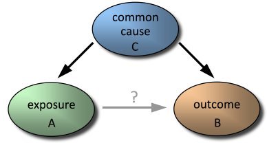
It is not easy to understand which independent variables I can make a significant contribution to the correctness of the forecast. The most logical way is to find those variables that would explain most of the deviations regarding the dependent variables. This approach is called best-subset.- search for the subset of variables that best predict responses to the dependent variable. An alternative is to find eigenvectors (a linear combination of available variables) that are responsible for deviations in the dependent variables. Typically, this approach is used in conjunction with the principal component analysis (PCA). The problem with him is that he can over-match the data. And finally, you can add variables to your model multiple times. This approach is used in multiple linear regression and in adaptive neural networks.

Conclusion

To create a model that would not produce some kind of distortion is almost impossible.
Even if the trader involved in developing the strategy manages to avoid the mistakes described above, the human factor still remains. Because someone will use the model - even if it is its author.

However, the important point here is that despite all the disadvantages and inaccuracies, some models are still useful and work better than others.

Can all financial models be wrong: 7 sources of risk of loss / ITI Capital Blog