Pandasql vs Pandas for solving data analysis problems
What are you talking about?
In this article, I would like to talk about the use of the Pandasql python library .
Many people who are faced with data analysis tasks are most likely familiar with the Pandas library . Pandas allows you to quickly and conveniently work with tabular data: filter, group, join on data; build pivot tables and even draw graphs (for simple visualization, the plot () function is enough , and if you want something more detailed, the matplotlib library will help ). On Habré repeatedly spoke about the use of this library for working with data: one , two , three .
But in my experience, not everyone knows about the Pandasql library, which allows you to work with Pandas DataFrames as tables and access them using the SQL language. In some tasks, it is easier to express what you want using the declarative language SQL, so I think that it is useful for people working with data to know about the availability of such functionality. If we talk about real problems, then I used this library to solve the join'a task of tables according to fuzzy conditions (it was necessary to combine records of events from different systems at approximately the same time, a gap of about 5 seconds).
Consider the use of this library with specific examples.
Data for analysis
To illustrate, I took data on the involvement of students in the Data Analyst Nanodegree specialization in Udacity. These data are published in the Intro to Data Analysis course (I can recommend this course to anyone who wants to get acquainted with using the Pandas and Numpy libraries for data analysis, although the Pandasql library is not considered there at all).
In the examples I will use 2 tables (more information about the data can be found here ):
- enrollments : data on the entry for the "Data Analyst Nanodegree" specialization of some random subset of students;
- account key : student ID;
- join date : the day the student signed up for a specialization;
- status : student status at the time of data collection: "current" if the student is active, and "canceled" if he left the course;
- cancel date : the day the student left the course, None for active students;
- is udacity : set to True for test accounts in Udacity, for live users - False;
- daily engagements : data on student activity from the enrollments table for each day when they were registered for specialization;
- acct : student ID;
- utc date : date of activity;
- total minutes visited : The total number of minutes a student spent in the Data Analyst Nanodegree specialization courses.
Examples
Now we can proceed to consider the examples. It seems to me that it will most clearly show how to solve each of the problems using the standard functionality of Pandas and Pandasql.
First you need to do all the necessary imports and load the data from the csv files into DataFrames. The full sample code and source data can be found in the repository .
import pandas as pd
import pandasql as ps
from datetime import datetime
import seaborn
daily_engagements = pd.read_csv('./data/daily_engagement.csv')
enrollments = pd.read_csv('./data/enrollments.csv')
Import of the seaborn library is used only to make the graphics more beautiful, no special library functionality will be used.
Simple request
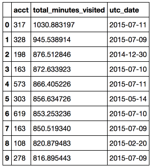
Task : find the top 10 maximum student activities on a particular day.
This example describes how to use filtering, sorting, and retrieving the N first objects. To execute a SQL query using the function
sqldfmodule Pandasql, and in this function it is necessary to convey Dictionary local names locals()(for more details about the use of functions locals()and globals()in Pandasql can be read on Stackoverflow ).# pandas code
top10_engagements_pandas = daily_engagements[['acct', 'total_minutes_visited', 'utc_date']]
.sort('total_minutes_visited', ascending = False)[:10]
# pandasql code
simple_query = '''
SELECT
acct,
total_minutes_visited,
utc_date
FROM daily_engagements
ORDER BY total_minutes_visited desc
LIMIT 10
'''
top10_engagements_pandas = ps.sqldf(simple_query, locals())Conclusion: The most diligent student spent more than 17 hours on the same day studying.
Using aggregate functions
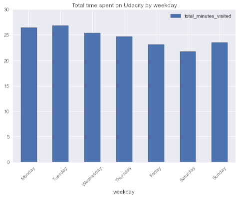
Objective : I wonder if there is a weekly seasonality in students' activity (judging by themselves, there is usually not enough time for online courses on weekdays, but you can spend more time on weekends).
First, add the weekday column to the original DataFrame, converting the date to the day of the week.
daily_engagements['weekday'] = map(lambda x: datetime.strptime(x, '%Y-%m-%d').strftime('%A'),
                                    daily_engagements.utc_date)
daily_engagements.head()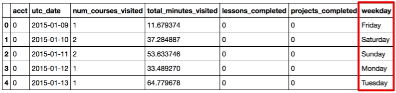
# pandas code
weekday_engagement_pandas = pd.DataFrame(daily_engagements.groupby('weekday').total_minutes_visited.mean())
# pandasql code
aggr_query = '''
    SELECT
        avg(total_minutes_visited) as total_minutes_visited,
        weekday
    FROM daily_engagements
    GROUP BY weekday
    '''
weekday_engagement_pandasql = ps.sqldf(aggr_query, locals()).set_index('weekday')
week_order = ['Monday', 'Tuesday', 'Wednesday', 'Thursday', 'Friday', 'Saturday', 'Sunday']
weekday_engagement_pandasql.loc[week_order].plot(kind = 'bar', rot = 45,
                                title = 'Total time spent on Udacity by weekday')
Conclusion: It is curious, but on average, students spend most of their time on courses on Tuesday, and least of all on Saturday. On average, students spend more time on MOOC on weekdays than on weekends. Another piece of evidence that I'm not representative.
JOIN tables
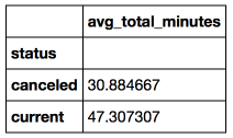
Objective : consider students who have not completed their specialization (with canceled status) and those who successfully study / studied and compare for them the average activity per day for the first week after they signed up for specialization. There is a hypothesis that those who stayed and study successfully spent more time learning.
To answer this question, we need data from both the enrollments and daily engagements tables , so we will use join by student ID.
Also in this problem there are several pitfalls to consider:
- not all users are living people, there are also Udacity test accounts, they need to be filtered
is_udacity = 0; - a student can register for specialization several times, including with an interval of less than one week, so you need to check that the activity date utc date is between join date and cancel date (only for students with canceled status).
# pandas code
join_df = pd.merge(daily_engagements,
                   enrollments[enrollments.is_udacity == 0],
                   how = 'inner',
                   right_on ='account_key',
                   left_on = 'acct')
join_df = join_df[['account_key', 'status', 'total_minutes_visited', 'utc_date', 'join_date', 'cancel_date']]
join_df['days_since_joining'] = map(lambda x: x.days,
                                    pd.to_datetime(join_df.utc_date) - pd.to_datetime(join_df.join_date))
join_df['before_cancel'] = (pd.to_datetime(join_df.utc_date) <= pd.to_datetime(join_df.cancel_date))
join_df = join_df[join_df.before_cancel | (join_df.status == 'current')]
join_df = join_df[(join_df.days_since_joining < 7) & (join_df.days_since_joining >= 0)]
avg_account_total_minutes = pd.DataFrame(join_df.groupby(['account_key', 'status'], as_index = False)
                                                 .total_minutes_visited.mean())
avg_engagement_pandas = pd.DataFrame(avg_account_total_minutes.groupby('status').total_minutes_visited.mean())
avg_engagement_pandas.columns = []
# pandasql code
join_query = '''
    SELECT
        avg(avg_acct_total_minutes) as avg_total_minutes,
        status
    FROM
        (SELECT
            avg(total_minutes_visited) as avg_acct_total_minutes,
            status,
            account_key
        FROM
            (SELECT
                e.account_key,
                e.status,
                de.total_minutes_visited,
                (cast(strftime('%s',de.utc_date) as interger) - cast(strftime('%s',e.join_date) as interger))/(24*60*60)
                                                                                                    as days_since_joining,
                (cast(strftime('%s',e.cancel_date) as interger) - cast(strftime('%s', de.utc_date) as interger))/(24*60*60)
                                                                                                    as days_before_cancel
            FROM enrollments as e JOIN daily_engagements as de ON (e.account_key = de.acct)
            WHERE (is_udacity = 0) AND (days_since_joining < 7) AND (days_since_joining >= 0)
                AND ((days_before_cancel >= 0) OR (status = 'current'))
            )
        GROUP BY status, account_key)
    GROUP BY status
'''
avg_engagement_pandasql = ps.sqldf(join_query, locals()).set_index('status')
It should be noted that SQL query function was used
castand strftimethat lines lead from a date timestamp (the number of seconds since the epoch) and then calculate the difference between these two dates in days. Conclusion: On average, students who did not give up their specialization spent 53% more time on Udacity in the first week than those who decided to stop studying.
Summarizing
In this article, we looked at examples of using the Pandasql library for data analysis and compared it using the Pandas functionality. We used filtering, sorting, aggregate functions and joins to work with DataFrames in Pandasql.
Pandas is a very convenient library that allows you to quickly and easily convert data, but it seems to me that in some tasks it is easier to express your thoughts using a declarative language and then Pandasql comes to the rescue. In addition, Pandasql can be useful for those who are just starting out with Pandas, but already have good knowledge of SQL.
Full sample code and source data are also provided in the github repository .
For those interested, there is also a good Pandasql tutorial on The Yhat Blog .